"I have watched you for two hundred mornings. The coffee shop on Tuesday, the gym on Thursday, the long way home when it rains. You think tonight is a free choice. I have already weighted the seven places you might go, and six of them I can name. The seventh is where you surprise yourself, and even that, I am learning."
A Trajectory That Knows Where You Are Going Before You Do
Every temporal model in this book so far has tracked a signal through time alone. Mobility data adds a second axis: a signal indexed by both where and when, a person or vehicle or disease tracing a path through space as the clock advances. A trajectory is a sequence of locations, and that single observation unlocks the entire machinery of Part III: next-location prediction is next-token prediction with a map instead of a vocabulary, and the same recurrent, convolutional, and attention models you built for text and sensors apply almost verbatim once you decide how to turn continuous coordinates into discrete tokens. The twist that makes mobility its own discipline rather than a relabeled sequence problem is the spatial structure layered on top of time: locations are not arbitrary symbols but points on a surface with distance, adjacency, and a road network connecting them, and good models exploit that geometry. This section establishes what spatio-temporal data is, frames human mobility as a sequence-modeling task, surveys the three ways to represent space (grids, graphs, and continuous coordinates), tours the applications from ride-hailing demand to epidemic spread, and closes by building a next-location predictor twice: a Markov model from scratch over discretized cells, then the same task in a few library lines. You leave able to take raw latitude-longitude pings and produce a calibrated guess at where the trace is going next, the foundation for every spatio-temporal system in this chapter.
Chapters 30 and 31 built temporal systems that reason and act: the causal reasoners of Chapter 30 and the temporal agents of Chapter 31 both treated the world as something unfolding in time. This chapter adds the dimension those systems were implicitly missing, namely space, and it does so by starting with the most human of spatio-temporal signals: where people go. The reason mobility opens the chapter rather than, say, weather grids is pedagogical. A trajectory is the cleanest bridge from the pure sequence models of Part III to the spatial world, because a trajectory is a sequence, just one whose tokens happen to be places. Everything you learned about modeling order, dependence, and prediction transfers directly; the only new ingredient is the geometry of the token space, and introducing that geometry one piece at a time is exactly what this section does.
Why does mobility deserve a foundational section of its own? Because it is simultaneously enormously valuable, surprisingly tractable, and genuinely subtle. Valuable: ride-hailing dispatch, public-transit planning, retail siting, epidemic response, and logistics all rest on predicting where demand and people will be. Tractable: human movement, far from being the free improvisation it feels like from the inside, is among the most predictable signals in all of behavioral science, a fact we will quantify precisely. Subtle: the spatial structure means a naive sequence model that ignores geometry leaves real signal on the table, and the privacy stakes of modeling individual movement are high enough that Chapter 33 devotes attention to them. Getting mobility right means holding the sequence view and the spatial view in mind at once.
The four competencies this section installs are these: to recognize a spatio-temporal field and write it down formally; to frame next-location prediction as a sequence task and connect it to the gravity and radiation models that long predated deep learning; to choose among grid, graph, and continuous representations of space for a given problem; and to build a working next-location predictor end to end, from raw pings to a transition-probability table, by hand and with a library. These are the load-bearing skills for the traffic forecasting of Section 32.2 and everything after.

1. Spatio-Temporal Data: Signals Indexed by Space and Time Beginner
Up to this point a time series has been a function of one variable: a value, or a vector of values, indexed by time $t$. Spatio-temporal data generalizes that by one axis. The fundamental object is a field $z$ that depends on both a spatial location $\mathbf{s}$ and a time $t$, written
$$z : \mathcal{S} \times \mathcal{T} \;\to\; \mathbb{R}^{d}, \qquad z(\mathbf{s}, t),$$where $\mathcal{S}$ is the spatial domain (a region of the plane, a set of grid cells, the nodes of a road graph) and $\mathcal{T}$ is the time domain. A single reading $z(\mathbf{s}, t)$ might be the traffic speed at intersection $\mathbf{s}$ at minute $t$, the number of taxi pickups in city block $\mathbf{s}$ during hour $t$, or the infection count in county $\mathbf{s}$ on day $t$. Fix the time and you have a spatial snapshot, a map; fix the location and you have an ordinary time series, the kind Parts II and III modeled. Spatio-temporal modeling is the art of using both slices at once: a value is correlated with its own past (temporal dependence, the whole of this book so far) and with the values at nearby locations (spatial dependence, the new ingredient), and usually with the recent past of nearby locations as well (the genuinely spatio-temporal interaction).
It helps to separate spatio-temporal data into two broad shapes, because they call for different machinery. The first is the field or raster shape just described, where space is partitioned into fixed cells or sensors and we observe a value in every cell at every timestep: traffic-sensor grids, weather rasters, pollution maps. Here $\mathcal{S}$ is fixed and the data is a tensor of shape (locations $\times$ time $\times$ channels), and the spatial structure is a grid or a graph over those fixed locations. The second is the trajectory or event shape, where the data is a set of moving entities each leaving a sequence of (location, time) stamps: GPS traces, check-ins, vehicle paths. Here the locations are not fixed cells but a continuous or discretized path through space, and each entity is a variable-length sequence. This section concentrates on the trajectory shape because it is the cleanest sequence problem; Section 32.2 takes up the field shape with traffic forecasting.
The entire conceptual jump from time series to spatio-temporal data is the addition of a single spatial axis $\mathbf{s}$ to the index. But that one axis introduces two correlations the temporal models did not have to model: spatial correlation (Tobler's first law of geography, "everything is related to everything else, but near things are more related than distant things"), and the cross term, where a location's future depends on its neighbors' recent past (congestion spilling from one road to the next, infection crossing a county line). A pure time-series model applied independently per location captures the first axis and ignores both new correlations, which is exactly the signal a spatio-temporal model is built to recover. Hold this in mind: spatio-temporal modeling is time-series modeling plus the question "what are the neighbors doing?".
A trajectory, the object at the center of this section, is the trajectory shape made precise. For one moving entity it is a time-ordered sequence of spatio-temporal points
$$\mathcal{P} = \big[(\mathbf{s}_1, t_1), (\mathbf{s}_2, t_2), \dots, (\mathbf{s}_n, t_n)\big], \qquad t_1 < t_2 < \cdots < t_n,$$where each $\mathbf{s}_i \in \mathcal{S}$ is a location (a latitude-longitude pair, a grid cell, a venue) and $t_i$ its timestamp. When the timestamps are dropped and only the order is kept, $\mathcal{P}$ collapses to a plain sequence of locations $[\mathbf{s}_1, \dots, \mathbf{s}_n]$, which is the form most next-location models consume. The timestamps still matter (people move differently at 8 a.m. and 8 p.m.) and good models keep them as features, but the skeleton is a sequence of places, and that skeleton is the bridge to Part III. Figure 32.1.1 shows the three shapes of spatio-temporal data side by side.
2. Human Mobility as a Sequence Modeling Task Beginner
Strip the timestamps from a trajectory and you have a sequence of locations $[\ell_1, \ell_2, \dots, \ell_n]$, each $\ell_i$ drawn from a finite vocabulary of places (cells, venues, or stay-points). The central predictive task, next-location prediction, is then stated in a form that should look extremely familiar after Part III: given the history, estimate the distribution over the next location,
$$P(\ell_{n+1} = \ell \mid \ell_1, \ell_2, \dots, \ell_n).$$This is next-token prediction. The vocabulary is a set of places instead of a set of words, but the object is identical: a conditional distribution over a discrete next symbol given a sequence of past symbols, exactly the quantity the neural sequence models of Chapter 9 were built to estimate and the backpropagation-through-time of Section 9.3 learns to fit. Every architecture from Part III therefore applies: a Markov model uses a fixed-order history, an RNN or LSTM (Chapter 10) carries an unbounded hidden state, and a Transformer (Chapter 12) attends over the whole visit history. The state of the art in next-location prediction is, unsurprisingly, attention-based, and it differs from a language Transformer mainly in how it injects spatial and temporal structure (distance between candidate locations, hour-of-day, day-of-week) as features rather than treating places as arbitrary tokens.
Before deep sequence models, mobility had a rich tradition of physical models that predicted flows between places from first principles, and they remain strong baselines and excellent priors. The oldest is the gravity model, which by analogy with Newtonian gravity predicts the flow $T_{ij}$ from place $i$ to place $j$ as growing with the two populations and decaying with distance:
$$T_{ij} \;\propto\; \frac{m_i\, m_j}{f(d_{ij})}, \qquad f(d_{ij}) = d_{ij}^{\beta} \ \text{or}\ e^{\beta d_{ij}},$$where $m_i, m_j$ are the masses (populations, or trip-generating capacities) of the two places, $d_{ij}$ is the distance between them, and $f$ is a deterrence function with a fitted exponent $\beta$. The gravity model is a workhorse of transport planning, but it has a known weakness: it requires the distance exponent to be tuned per region and does not transfer well. The radiation model (Simini and colleagues, 2012) replaced the tunable physics with a parameter-free probabilistic argument: a traveler from $i$ accepts the nearest destination whose attractiveness exceeds the best opportunity available closer to home, which yields
$$\langle T_{ij} \rangle \;=\; T_i \, \frac{m_i\, m_j}{(m_i + s_{ij})(m_i + m_j + s_{ij})},$$where $s_{ij}$ is the total mass in the circle of radius $d_{ij}$ centered at $i$ (the intervening opportunities) and $T_i$ is the total outflow from $i$. The radiation model has no free parameters and predicts aggregate commuting flows remarkably well, which is why it is the standard physical baseline against which learned mobility models are measured.
In Chapter 1 we met the result that bounds every forecaster: Song, Qu, Blumm, and Barabasi (2010) measured the entropy of human trajectories from months of mobile-phone records and found a theoretical maximum predictability of about 93 percent for a typical person's next location. That number is one of the most cited facts in mobility science, and it is precisely a limits-of-predictability statement of the kind Section 1.5 framed in general: it says the entropy of where-you-go-next is low, that despite the feeling of free choice your movement is dominated by a handful of habitual places, and that no model, however clever, can exceed roughly 93 percent accuracy on the population average. Mobility is the cleanest real-world illustration of that chapter's thesis: the predictability ceiling is high because the signal is regular, and the gap between a simple Markov model (often 70 to 80 percent) and that ceiling is the room learned models compete in.
That high predictability is the single most important fact about human mobility for a modeler, and it is worth pausing on why it holds. People are creatures of routine: most of anyone's movement is among a small set of frequently visited places (home, work, a few regular shops and social spots), the visits follow strong daily and weekly cycles, and transitions between places are highly structured (you go home from work far more often than you go to a random venue). All three regularities, a small effective vocabulary, strong periodicity, and structured transitions, are exactly the properties that make a sequence highly compressible and therefore highly predictable. The practical consequence is that even a crude model does well, which sets a high floor and means the interesting competition is in the last several percentage points, where capturing context (it is Friday evening, it is raining, you just left a restaurant) separates a good model from a great one.
The unsettling charm of the 93 percent result is that it holds regardless of how much you travel. The original study found that people who roam over large areas are no less predictable than homebodies: a frequent traveler simply has a larger but equally habitual set of haunts. Your sense of spontaneity is real to you and nearly invisible to the data. The model in subsection five will, on synthetic routine data, happily predict your evening with the smug confidence of someone who has read your calendar, because in a statistical sense it has. The seventh place, the genuinely surprising one, is the entropy the ceiling leaves on the table, and chasing it is what keeps mobility modeling an open problem rather than a solved one.
3. Representing Space: Grids, Graphs, and Coordinates Intermediate
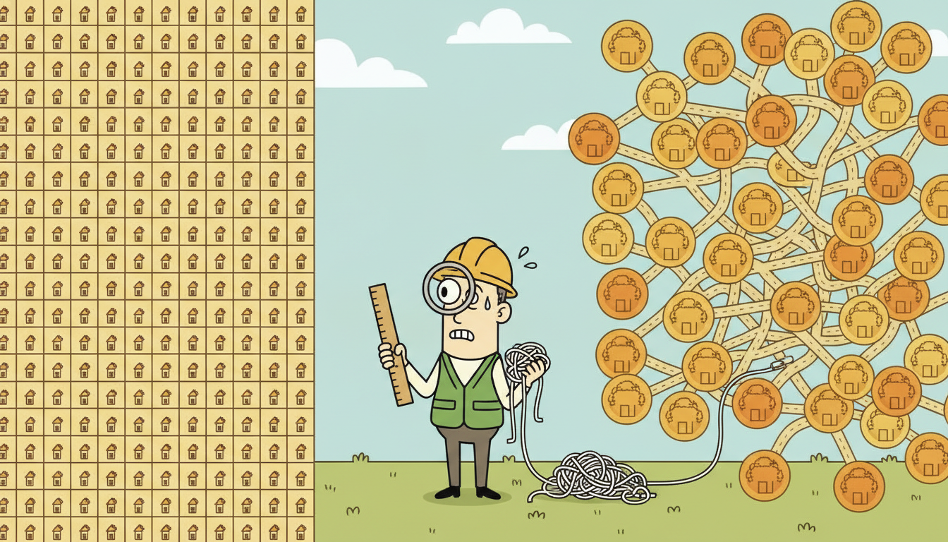
Before any model touches a trajectory, a representational decision has to be made: how is a location encoded? Continuous latitude-longitude is the raw form, but most models need a discrete or structured representation, and the choice shapes everything downstream. There are three dominant options, and they correspond to three different ways of imposing geometry on the sequence vocabulary.
The first is the grid or tessellation: partition the surface into cells and replace each coordinate with the cell that contains it. The simplest is a uniform rectangular grid, but the geospatial standards are hierarchical and global. Geohash interleaves latitude and longitude bits into a base-32 string, so a longer string is a smaller cell and a shared prefix means spatial proximity, which makes prefix matching a cheap proximity test. H3 (Uber's hexagonal hierarchical index) tiles the globe with hexagons at sixteen resolutions; hexagons are preferred over squares because every neighbor is equidistant (squares have nearer edge-neighbors and farther corner-neighbors), which makes neighbor-aggregation cleaner. Gridding turns the location vocabulary finite and gives every cell a set of well-defined neighbors, at the cost of a resolution choice: too coarse and you blur distinct places together, too fine and the vocabulary explodes and each cell is visited too rarely to estimate.
The second is the graph: represent space as the nodes and edges of a network, most naturally the road network, where nodes are intersections or road segments and edges encode physical connectivity. A trajectory becomes a walk on this graph (map-matching snaps noisy GPS pings to the most likely path along the edges), and the graph's adjacency is the correct notion of spatial proximity for anything that travels on roads, because two points can be close in straight-line distance yet far along the network (opposite banks of a river, two sides of a highway). Graph representations pair naturally with graph neural networks, which we meet for traffic in Section 32.2.
The third is to keep continuous coordinates and learn a spatial embedding: a function that maps a latitude-longitude (or a cell index) to a dense vector, trained so that places that play similar roles in trajectories land near each other in embedding space, exactly as word embeddings place similar words together. This is the dominant choice inside neural next-location models: each location id is mapped through an embedding table (or each coordinate through a small network, sometimes with sinusoidal position-style encodings of latitude and longitude) into a vector that the sequence model consumes. The embedding learns geometry the discrete vocabulary threw away, so two cells that are different tokens but functionally interchangeable get similar vectors. Figure 32.1.2 contrasts the three representations.
| Representation | Location becomes | Proximity is | Strength | Watch out for |
|---|---|---|---|---|
| Grid / tessellation (geohash, H3) | a cell id from a finite set | shared prefix / hex adjacency | finite vocabulary, global, hierarchical | resolution trade-off; sparse cells |
| Graph (road network) | a node or edge of a network | network adjacency | respects real connectivity | needs map-matching; build cost |
| Continuous + embedding | a learned dense vector | distance in embedding space | learns latent geometry; feeds neural nets | needs data to train; less interpretable |
The standard recipe in modern mobility modeling is a two-step move that resolves the tension between "sequence models want discrete tokens" and "space is continuous and geometric". First discretize (grid the surface into H3 cells or snap to road nodes) so the location vocabulary is finite and the problem becomes next-token prediction. Then embed (learn a dense vector per cell) so the geometry the discretization threw away is recovered as learned similarity. Discretization makes the problem a sequence problem; embedding makes the sequence problem spatially aware. Skipping the second step gives you a model that treats two adjacent cells as no more related than two cells across the city, which is the classic mistake of applying a text model to places without telling it that places have a map.
4. Applications: Demand, Disease, Logistics, and Recommendation Intermediate
Mobility modeling earns its keep across a striking range of domains, and seeing the spread clarifies why the field invests so heavily in it. Demand prediction is the flagship: ride-hailing and delivery platforms forecast, for each region and each upcoming time window, how many requests will originate there, so vehicles can be repositioned ahead of demand. This is a spatio-temporal field-forecasting problem (predict a value per cell per future step) and it sits at the heart of the dispatch systems that make the difference between a five-minute and a fifteen-minute wait. Epidemic spread turns mobility into an input for compartmental and metapopulation models: where people travel determines where a pathogen goes, and the mobility matrices estimated by gravity and radiation models (and, increasingly, by phone-derived flows) feed directly into the differential equations that forecast outbreaks, a use that became globally visible during recent pandemics.
Logistics applies the same machinery to fleets and freight: predicting where vehicles and shipments will be, routing them efficiently, and anticipating congestion, which connects mobility to the optimal-control and planning ideas of Chapter 27. Location recommendation is the consumer-facing cousin of next-location prediction: given where a user has been, suggest where they might want to go next (the next restaurant, the next point of interest), which is next-location prediction repackaged as a ranking task and powers the "places you might like" features in mapping and review apps. Across all four, the common core is the same conditional distribution over future spatio-temporal states that this section builds.
Who: The marketplace team at a regional ride-hailing company operating a few thousand drivers across one metro area.
Situation: Riders requested cars from their phones; the dispatch system matched each request to the nearest free driver. At peak times, demand surged in districts (a stadium after a game, a business district at 6 p.m.) faster than idle drivers could drift toward them, so riders in those districts waited while drivers sat idle elsewhere.
Problem: They needed to forecast, fifteen to thirty minutes ahead and per H3 cell, how many requests would originate, so they could nudge idle drivers toward soon-to-be-hot cells before the surge rather than chasing it.
Dilemma: A pure per-cell time-series model (one forecaster per cell, Part II style) ignored that a surge in one district is preceded by movement out of its neighbors, and it had nothing to say about cells with sparse history. A single global sequence model risked smearing very different districts together.
Decision: They gridded the city to H3 resolution-8 cells, learned an embedding per cell, and trained a spatio-temporal model that predicted each cell's next-window demand from its own recent history and its neighbors' (the cross term of subsection one), with hour-of-day and day-of-week features.
How: Demand per cell per five-minute bin became the field; the model consumed a short window of recent bins across a cell and its H3 ring of neighbors; predictions drove a repositioning recommender that suggested target cells to idle drivers.
Result: Median rider wait in the previously underserved peak districts fell by a meaningful margin because cars arrived ahead of demand, and idle-driver time dropped because drivers were steered toward genuine upcoming demand rather than the last surge.
Lesson: Demand prediction is spatio-temporal, not per-cell-temporal: the neighbors' recent past carries the early warning, and gridding plus embedding plus a neighbor-aware model is the standard recipe. A per-cell forecaster leaves the most valuable signal, the spatial spillover, entirely unused.
One application cuts the other way and must be named plainly: modeling individual movement is modeling people, and a trajectory is among the most sensitive data a person generates. Where you sleep, work, worship, seek medical care, and protest are all legible in a few weeks of location pings, and even "anonymized" trajectories are notoriously re-identifiable because a handful of visited places uniquely fingerprints a person. The techniques of this section are dual-use, and the responsible-AI treatment of privacy, including differential privacy and the re-identification risk of trajectory data, is taken up directly in Chapter 33. We flag it here so that no reader leaves this section thinking the only question mobility raises is accuracy.
The most active recent thread mirrors what happened to language and to time series in Chapter 15: large pretrained models for mobility. Work since 2023 has trained Transformer-based next-location predictors at scale and probed whether large language models can reason about trajectories directly, with systems such as LLM-Mob and the broader "LLMs for mobility" line (2023 to 2024) reformulating next-location prediction as a prompting task over textualized visit histories, and dedicated trajectory foundation models pretrained on massive GPS corpora, such as the UniMob line of universal mobility models (2025), aiming for the zero-shot transfer across cities that single-city models lack. In parallel, generative mobility has advanced: diffusion and other generative models now synthesize realistic trajectories (work around 2023 to 2025) for data augmentation and, crucially, for privacy, producing synthetic populations that preserve aggregate statistics without exposing real individuals, which ties directly to the differential-privacy concerns of Chapter 33. The 2026 open questions are the familiar foundation-model ones, transfer across cities and modalities and faithful long-horizon generation, now sharpened by mobility's unique privacy stakes.
5. Worked Example: A Next-Location Predictor, From Scratch and By Library Advanced
We now build the simplest honest next-location predictor end to end: a first-order Markov model over discretized cells. The plan mirrors the from-scratch-then-library pattern used throughout the book. First we synthesize routine trajectories, discretize the continuous coordinates to a grid, estimate the transition-probability matrix by counting, and evaluate top-1 next-cell accuracy by hand. Then we do the same task with scikit-mobility, the standard Python mobility library, and count the lines saved. Code 32.1.1 generates synthetic routine trajectories and discretizes them.
import numpy as np

rng = np.random.default_rng(7)

# A tiny "city": 5 named places at fixed coordinates (lon, lat in arbitrary units).
places = {0: (0.1, 0.1),   # home
          1: (0.8, 0.2),   # work
          2: (0.5, 0.7),   # gym
          3: (0.2, 0.6),   # cafe
          4: (0.9, 0.9)}   # friend
coords = np.array([places[i] for i in range(5)])

# A routine: a habitual transition matrix (rows sum to 1). People are predictable:
# from home you usually go to work or cafe; from work you usually go home, etc.
P_true = np.array([
    [0.05, 0.55, 0.10, 0.25, 0.05],   # from home
    [0.60, 0.05, 0.20, 0.05, 0.10],   # from work
    [0.50, 0.10, 0.05, 0.30, 0.05],   # from gym
    [0.55, 0.20, 0.15, 0.05, 0.05],   # from cafe
    [0.45, 0.15, 0.10, 0.25, 0.05]])  # from friend

def sample_trajectory(n_steps, start=0):
    """Walk the routine chain, emitting a noisy GPS ping near each chosen place."""
    seq, pings = [start], []
    for _ in range(n_steps):
        nxt = rng.choice(5, p=P_true[seq[-1]])     # habitual next place
        seq.append(nxt)
    for p in seq:
        pings.append(coords[p] + rng.normal(0, 0.03, size=2))  # GPS noise
    return seq, np.array(pings)

# 200 routine days, ~12 stops each: our raw trajectory corpus of noisy (lon, lat) pings.
all_pings, all_truth = [], []
for _ in range(200):
    seq, pings = sample_trajectory(12)
    all_pings.append(pings); all_truth.append(seq)

# Discretize: snap each continuous ping to its nearest grid cell (here, nearest place).
def to_cells(pings):
    d = ((pings[:, None, :] - coords[None, :, :]) ** 2).sum(-1)  # sq dist to each cell
    return d.argmin(1)                                            # nearest-cell id

cell_seqs = [to_cells(p) for p in all_pings]
print("first trajectory, cells:", cell_seqs[0][:8])
print("total visits:", sum(len(s) for s in cell_seqs))
P_true drives a Markov walk over five places; each visit emits a noisy GPS ping; to_cells snaps every continuous ping back to its nearest grid cell, the discretize-to-tokenize step of subsection three. The output is a corpus of integer location sequences ready for next-location modeling.first trajectory, cells: [0 1 0 3 0 1 2 0]
total visits: 2600
With discrete sequences in hand, the model is a transition table estimated by counting: $\hat{P}(\ell' \mid \ell)$ is the fraction of times cell $\ell$ was followed by cell $\ell'$. Prediction is then "take the most likely successor of the current cell". Code 32.1.2 estimates the matrix, evaluates top-1 accuracy on held-out trajectories, and reads off one transition probability for the numeric callout.
n_cells = 5
split = 160
train, test = cell_seqs[:split], cell_seqs[split:]

# Estimate the transition matrix by counting consecutive (current -> next) pairs.
counts = np.zeros((n_cells, n_cells))
for seq in train:
    for cur, nxt in zip(seq[:-1], seq[1:]):
        counts[cur, nxt] += 1
P_hat = counts / counts.sum(1, keepdims=True)        # row-normalize to probabilities

# Predict: the most likely successor of the current cell. Evaluate top-1 accuracy.
pred_next = P_hat.argmax(1)                           # argmax row -> predicted next cell
correct = total = 0
for seq in test:
    for cur, nxt in zip(seq[:-1], seq[1:]):
        correct += (pred_next[cur] == nxt)
        total += 1
print("estimated P(next | home):", np.round(P_hat[0], 3))
print("top-1 next-location accuracy: %.3f" % (correct / total))
estimated P(next | home): [0.05  0.557 0.099 0.244 0.05 ]
top-1 next-location accuracy: 0.638
The estimated row P_hat[0] for "from home" came out as $[0.05,\ 0.557,\ 0.099,\ 0.244,\ 0.05]$ over the five cells (home, work, gym, cafe, friend). Read directly, this says: starting from home, the model assigns probability $\hat{P}(\text{work}\mid\text{home}) = 0.557$ to going to work next, $\hat{P}(\text{cafe}\mid\text{home}) = 0.244$ to the cafe, and only $0.05$ each to gym, friend, or staying. The argmax prediction is therefore work, and it is right whenever the person actually went to work, which the true matrix says happens 55 percent of the time. Notice the estimate $0.557$ is within a hundredth of the true $0.55$: with 160 training trajectories of about twelve stops, roughly two thousand transitions, the law of large numbers has pinned the common transitions tightly while the rare ones (the $0.05$ entries) are noisier. That the estimated row $0.557$ and $0.244$ recover the true $0.55$ and $0.25$ to within a hundredth is exactly the calibration evidence: the estimated probabilities match the empirical frequencies, so reading $\hat{P}(\text{work}\mid\text{home})$ as a real probability is justified, not just an argmax label. The single transition probability is the atom of the whole model: a next-location predictor is nothing but a calibrated table of these numbers, and a neural model is the same table made conditional on richer context.
Now the library equivalent. scikit-mobility (the skmob package) is the standard open-source toolkit for human-mobility analysis: it wraps trajectories in a TrajDataFrame, ships tessellation, stop-detection, gravity and radiation models, and privacy assessments, and turns the multi-step pipeline of Code 32.1.1 and 32.1.2 (synthesize, discretize, count, normalize, evaluate) into a handful of high-level calls. Code 32.1.3 sketches the same gridding-and-flow workflow with the library.
import pandas as pd
import skmob
from skmob.tessellation import tilers
from skmob.models.gravity import Gravity

# 1. Wrap raw pings as a TrajDataFrame (lat, lng, user id, timestamp): library's core type.
df = pd.DataFrame({"lat": all_pings[0][:, 1], "lng": all_pings[0][:, 0],
                   "uid": 0, "datetime": pd.date_range("2026-01-01", periods=12, freq="h")})
tdf = skmob.TrajDataFrame(df, latitude="lat", longitude="lng",
                          user_id="uid", datetime="datetime")

# 2. Tessellate space into a grid (the discretize step) with one call.
tessellation = tilers.tiler.get("squared", base_shape="London, UK", meters=1000)

# 3. Map points to cells, then fit a flow model (gravity) on the resulting OD flows.
mapped = tdf.mapping(tessellation)                    # snap each ping to its tile id
gravity = Gravity(gravity_type="singly constrained")  # the gravity model of subsection 2
# gravity.fit(flow_df, relevance_column="population") # fit on observed origin-destination flows
print(mapped.head())
TrajDataFrame holds the trajectory, tilers.tiler.get tessellates space, tdf.mapping performs the discretization that Code 32.1.1 wrote by hand, and Gravity provides the physical flow model of subsection two as a fitted object. The library also ships the radiation model and privacy-risk assessment as one-liners.The from-scratch pipeline of Code 32.1.1 and 32.1.2 ran roughly 40 lines: hand-rolled discretization, manual transition counting, row normalization, and an accuracy loop. scikit-mobility collapses the spatial plumbing to a few calls: TrajDataFrame ingests the trajectory, tilers.tiler.get plus tdf.mapping replace the entire nearest-cell discretization, and Gravity or Radiation provide the physical flow models of subsection two as fitted objects, where a from-scratch radiation model would be dozens of lines on its own. The library handles tessellation geometry, coordinate-reference systems, stop detection, and even privacy-risk assessment internally. The rule of this book holds: implement the Markov counter once by hand to own the idea, then reach for skmob (or PyTorch with a learned embedding for the neural version) for anything you intend to ship.
Read the three code blocks together as the section in miniature. Code 32.1.1 turned continuous GPS pings into discrete location tokens, the discretize-to-tokenize move of subsection three. Code 32.1.2 estimated the conditional next-location distribution of subsection two by counting and scored it, recovering the routine and landing well below the predictability ceiling of subsection two, which is exactly where a context-aware neural model earns its complexity. Code 32.1.3 showed the same spatial pipeline in a few library lines and surfaced the gravity model of subsection two as a fitted object. The Markov model is the floor; Section 32.2 raises the spatial structure to a graph and brings the neural machinery to bear on the field-shaped cousin of this problem, traffic.
Exercises
- Conceptual. A colleague proposes forecasting ride-hailing demand by fitting one independent ARIMA model per H3 cell (the Part II approach) and arguing that "each cell is just a time series". Using the field-shape definition and the cross-correlation term of subsection one, explain precisely what signal this per-cell approach cannot capture, and give a concrete city scenario (name the cells and the spillover) where ignoring that signal would make the forecast late. Then state what minimal change to the model would recover the missing signal.
- Implementation. Extend the from-scratch predictor of Code 32.1.2 from first-order to second-order: estimate $\hat{P}(\ell_{n+1}\mid \ell_n, \ell_{n-1})$ by counting consecutive triples, and predict the argmax successor of the current pair of cells. Re-run the held-out top-1 accuracy and compare it to the first-order baseline of 0.638. Then explain, in terms of the small-vocabulary-and-sparse-counts trade-off of subsection three, why second order helps on this five-place synthetic data but can hurt when the cell vocabulary is large and many pairs are never seen in training.
- Open-ended. The radiation model of subsection two is parameter-free, while the gravity model has a tunable distance exponent $\beta$. Design an experiment, on real or realistic synthetic origin-destination flow data, that would tell you which model better predicts commuting flows in a given region, and state in advance what result would make you prefer each. Discuss how the high individual-level predictability ceiling from Chapter 1 does or does not transfer to the aggregate flow-prediction setting these physical models target, and whether a learned mobility foundation model (subsection four's frontier) should be expected to beat both.