Predictability, Entropy Rate, and the Limits of Forecasting

"Some days I am a gentle drift you could forecast in your sleep. Other days I reinvent my own distribution out of spite. Please stop asking me what I will do next Tuesday; I genuinely do not know either."

A Non-Stationary Process Having an Identity Crisis

In Section 1.4 we classified temporal data along several axes, from regular univariate grids to irregular event streams, and saw that stationarity is the axis that governs how much the past can say about the future. That taxonomy quietly assumed the future was forecastable to begin with. It is time to confront the assumption head on. A forecasting project that begins by fitting an elaborate network to a series that is, in truth, indistinguishable from noise is not merely wasteful; it is actively dangerous, because a flexible model will always find spurious structure in finite samples and report a confidence it has not earned. This section equips you to measure forecastability first, so that the modeling chapters that follow are aimed at series that can actually reward the effort.

1. Signal Versus Noise: The Irreducible Innovation Beginner

Fix a stochastic process $\{X_t\}$ and stand at time $t-1$ with the entire observed past $X_{1:t-1} = (X_1, \dots, X_{t-1})$ in hand. The cleanest decomposition in all of forecasting writes the next value as a part the past explains plus a part it cannot:

The term $\mu_t$ is the best possible forecast under squared-error loss: among all functions of the past, the conditional expectation minimizes the expected squared error, a fact we develop fully alongside the unified notation of Appendix A. The term $\varepsilon_t$ is the innovation, the genuinely new information that arrives at time $t$ and that, by construction, is uncorrelated with everything knowable beforehand. Forecasting is, in its entirety, the project of recovering $\mu_t$. The innovation is the wall. No estimator, no amount of data, and no architecture from the later chapters of this book can predict $\varepsilon_t$, because it is defined as the residue that the past leaves undetermined.

The canonical illustration is the random walk, the process that will haunt every honest forecaster in this book. Let $X_t = X_{t-1} + \varepsilon_t$ with the innovations independent and identically distributed and zero-mean. Substituting into the decomposition, the conditional mean collapses to the last observed value:

so the provably optimal one-step forecast is simply "tomorrow equals today". The series wanders without bound, looks rich with apparent trends and reversals, and yet every visible pattern is an artifact of accumulated noise. This is why the random walk, and its drift-augmented cousin, serve as the naive baseline against which every model in Chapter 5 must justify its existence. A model that cannot beat "tomorrow equals today" has learned nothing real.

2. Entropy Rate: The Bit-Rate of Surprise Intermediate

Variance captures the size of the innovation under squared-error loss, but predictability is more naturally an information-theoretic quantity: how many bits of genuine surprise does each new observation carry, once the past is fully accounted for? The answer is the entropy rate. Recall that the Shannon entropy of a discrete block of observations measures its average uncertainty in bits,

where the sum runs over all possible length-$n$ trajectories. The entropy rate is the per-symbol limit of this block entropy as the window grows without bound:

For a stationary process this limit exists, and it admits a second, more operationally meaningful form. Instead of dividing total uncertainty by length, ask directly how uncertain the next symbol is given an ever-longer past:

These two definitions coincide for any stationary source, a theorem of Shannon that the further reading of Appendix B develops. The conditional form is the one to carry in your head: $h$ is the residual uncertainty about the next value that survives after conditioning on the entire history. It is the bit-rate of surprise, the irreducible information the future delivers that the past could never have supplied.

The two extremes anchor the intuition. For a perfectly predictable process, a fixed period-three cycle or a constant, the next symbol is determined by the past, the conditional entropy is zero, and so $h = 0$: no surprise, ever. For independent and identically distributed noise, the past tells you nothing, conditioning changes nothing, and $h$ equals the full per-symbol entropy $H(X)$, its maximal value. Every real series lives between these poles, and its entropy rate is precisely how far it sits from each. A low entropy rate is a promise that the series is forecastable; a high one is a warning.

3. The Predictability Ceiling: Bounds No Model Can Beat Advanced

Entropy rate would be an academic curiosity if it did not translate into a hard limit on achievable accuracy. It does. Consider forecasting a series quantized into $A$ possible symbols, and let $\Pi$ denote the probability that a forecaster correctly names the next symbol. Fano's inequality ties the entropy that remains to the error probability: if conditioning on the past leaves conditional entropy $H(X_n \mid X_{1:n-1})$, then any predictor's error rate $1 - \Pi$ must satisfy the inequality below. The illustration pictures this as a barrier no amount of cleverness can push through.

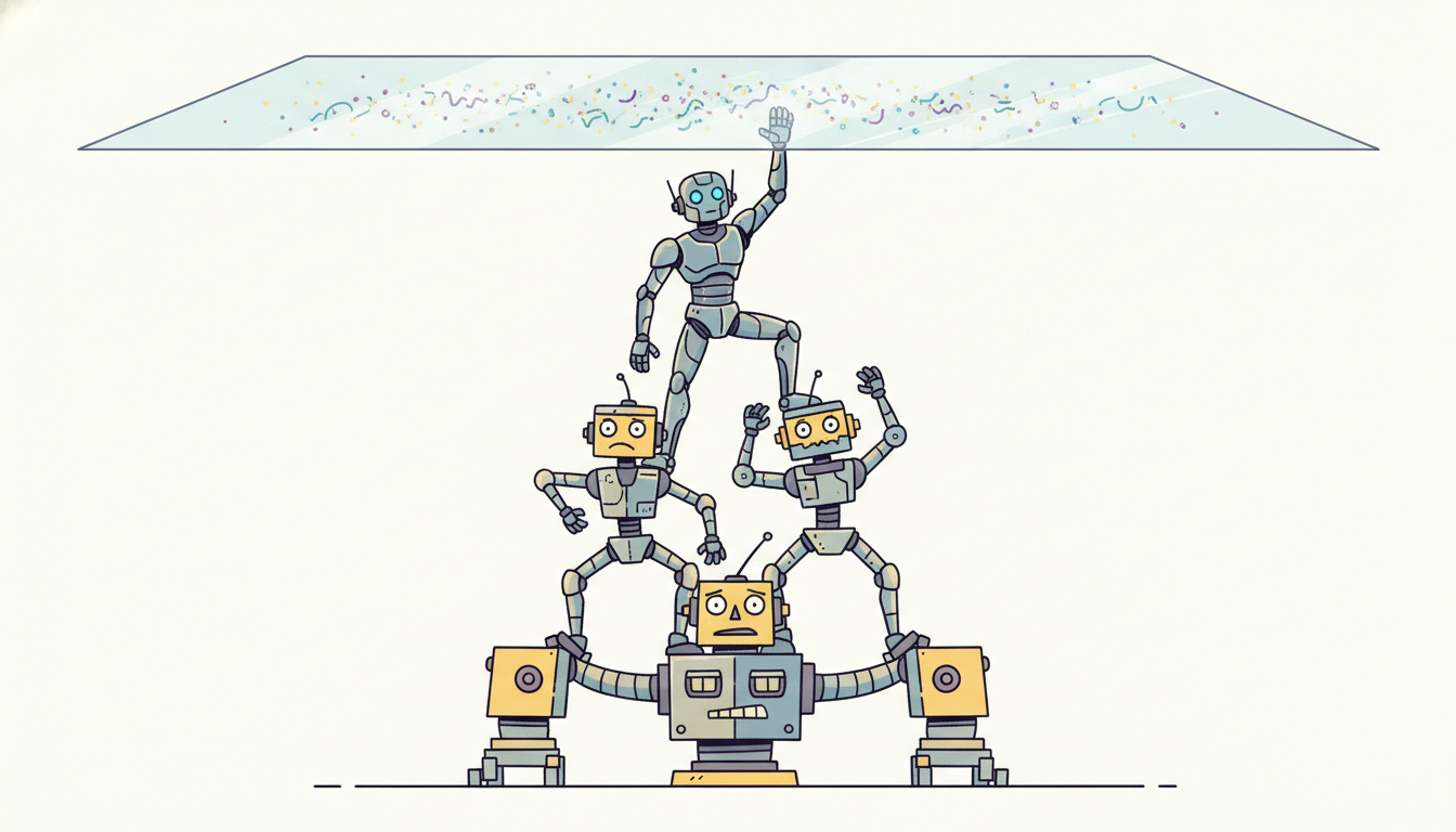
where $H_b(p) = -p \log_2 p - (1-p)\log_2(1-p)$ is the binary entropy function. The inequality runs one way: residual entropy forces a floor on the error, and therefore a ceiling on accuracy. Read it as a budget. The surprise that the past cannot remove has to show up somewhere, and the only place it can go is into forecasting mistakes. Inverting the bound for a fixed entropy rate $h$ and alphabet size $A$ yields the maximum predictability $\Pi_{\max}$, the largest fraction of correct one-step forecasts that any algorithm could attain on that source.

This is exactly the machinery that Song, Qu, Blumm, and Barabasi used in their 2010 study of human mobility, which estimated the entropy rate of where people go from anonymized phone records and solved Fano's bound for $\Pi_{\max}$. The result startled the field: across a large population, the typical $\Pi_{\max}$ was about $0.93$, meaning that the location of a regular human, an hour ahead, is in principle correctly predictable ninety-three percent of the time, regardless of how irregular individual people believe their schedules to be. The bound does not name the model that achieves it; it simply certifies that no model can exceed it. When a deployed system reports ninety percent accuracy on such a series, the right reaction is not "impressive" but "close to the ceiling, so further modeling will buy almost nothing".

4. Chaos: Deterministic Yet Unpredictable Advanced

Entropy rate frames unpredictability as randomness, the arrival of new information. There is a second, subtler source of unpredictability that needs no randomness at all: deterministic chaos. A chaotic system is governed by exact, noise-free equations, so in principle its entire future is fixed by its present state. Yet it is unpredictable in practice because it amplifies the tiniest uncertainty in that present state at an exponential rate. Two trajectories that start a distance $\delta_0$ apart separate, on average, as

where $\lambda$ is the largest Lyapunov exponent of the system. When $\lambda > 0$, any error in the initial condition, and you always have some, however small, grows until it dominates the signal. Suppose your knowledge of the present state carries an uncertainty $\delta_0$, and your forecast becomes useless once that uncertainty grows to a tolerance $\epsilon$. Setting $\delta_0 e^{\lambda t} = \epsilon$ and solving gives the prediction horizon

and the punchline is brutal: the horizon grows only as the logarithm of your measurement precision. To forecast twice as far ahead, you do not need twice the precision; you need to square it, an exponential improvement in instrumentation for a linear gain in reach. This is the mathematical reason weather forecasting has a wall at roughly two weeks. The atmosphere's largest Lyapunov exponent makes errors double every day or two, so even a perfect model fed near-perfect observations loses all skill after about a fortnight, and no satellite fleet will ever push that wall out by more than a few days.

The practical distinction between the two sources of unpredictability matters enormously for modeling strategy. Stochastic noise injects fresh information at every step, so its entropy rate is genuinely positive and no model can ever forecast past one step with the lost information recovered. Deterministic chaos injects nothing new; it merely magnifies old uncertainty, so a short-horizon forecast is achievable and worthwhile, and the entire goal becomes pushing $T_{\text{pred}}$ outward by reducing $\delta_0$ and by modeling the dynamics faithfully. A series that is chaotic but low-noise is forecastable in the short run and hopeless in the long run; a series that is high-entropy noise is hopeless even one step out. Telling these apart is the diagnostic work of the next subsection.

5. Practical Estimators of Forecastability Intermediate

The quantities above are limits over infinite data, so on a finite series we estimate them with practical proxies. Three families dominate. Permutation entropy converts the series into the relative-order patterns of short windows and measures the Shannon entropy of those ordinal patterns, a robust, almost parameter-free estimate that is high for noise and low for structured dynamics. Spectral entropy treats the normalized power spectrum as a probability distribution over frequencies and measures its entropy: a series whose energy concentrates at a few frequencies has low spectral entropy and is forecastable, while white noise spreads energy flat across all frequencies and saturates the entropy at its maximum. The third and simplest family is the beatability check: compute the error of a naive random-walk or seasonal-naive forecast, and ask whether any model improves on it at all. If nothing beats the naive baseline, the series is at the noise floor.

Code 1.5.1 builds a crude but honest forecastability diagnostic from scratch using spectral entropy, then contrasts a structured, predictable series against pure white noise so you can see the gap directly.

import numpy as np
from scipy import signal

def spectral_entropy(x, sf=1.0):
    """Normalized spectral entropy in [0, 1]: 0 = perfectly forecastable
    (energy at one frequency), 1 = white noise (energy spread flat)."""
    x = np.asarray(x, dtype=float)
    x = x - x.mean()                          # remove DC so it doesn't dominate
    freqs, psd = signal.periodogram(x, fs=sf) # power spectral density
    psd = psd[1:]                             # drop the zero-frequency bin
    p = psd / psd.sum()                       # treat the spectrum as a pmf
    p = p[p > 0]                              # log(0) guard
    H = -np.sum(p * np.log2(p))              # Shannon entropy of the spectrum
    return H / np.log2(len(p))               # normalize by the max possible

rng = np.random.default_rng(0)
n = 4096
t = np.arange(n)

# A predictable series: two clean periodicities plus a little noise.
predictable = (np.sin(2*np.pi*t/64) + 0.5*np.sin(2*np.pi*t/16)
               + 0.1*rng.standard_normal(n))
# The noise floor: an unforecastable i.i.d. Gaussian series.
white_noise = rng.standard_normal(n)

for name, x in [("structured signal", predictable),
                ("white noise", white_noise)]:
    se = spectral_entropy(x)
    # One-step naive (random-walk) forecast error vs. the series' own scale.
    naive_mae = np.mean(np.abs(np.diff(x)))
    print(f"{name:>18}: spectral_entropy={se:.3f}  naive_MAE={naive_mae:.3f}")

  structured signal: spectral_entropy=0.196  naive_MAE=0.184
        white noise: spectral_entropy=0.997  naive_MAE=1.357

The two numbers tell a consistent story. The structured series concentrates its energy in two spectral peaks, so its normalized spectral entropy is far below one and its step-to-step naive error is small, both signs that a forecaster has real structure to learn. The white-noise series spreads energy evenly across all frequencies, drives the spectral entropy to its ceiling, and leaves a large naive error that no model will reduce. Run this diagnostic before training anything: it costs milliseconds and can save weeks of fitting models to series that have nothing to teach them. For permutation entropy and a battery of related measures, the antropy and nolds libraries provide vetted implementations, as the shortcut below notes.

# Replace the 12-line spectral_entropy function with vetted estimators
# that also handle short series and ties in the ordinal patterns.
import antropy as ant

se = ant.spectral_entropy(predictable, sf=1.0, method="welch", normalize=True)
pe = ant.perm_entropy(predictable, order=3, normalize=True)  # ordinal-pattern
print(f"spectral={se:.3f}  permutation={pe:.3f}")

6. The Humbling Lesson and How to Use It Beginner

Put the pieces together and a sobering picture emerges. A great deal of real-world data, asset returns, ad-click rates, the next tick of many high-frequency processes, lives near its own noise floor, with an entropy rate close to maximal and a predictability ceiling barely above chance. On such series, the gap between a naive baseline and the theoretical optimum is so thin that a heroic modeling effort can claim, at best, a sliver of improvement, and will more often claim a fictitious one born of overfitting. The humbling lesson is that the question is not "which model is best?" but "is this series forecastable enough to be worth a model at all?", and that question has a measurable answer you can compute before you start.

Using the lesson well reshapes a project in three ways. First, it sets honest expectations: a forecast that reaches eighty-five percent of $\Pi_{\max}$ is excellent even if its raw accuracy sounds modest, while one that beats a random walk by a hair on a noise-floor series is almost certainly overfit. Second, it disciplines evaluation: every reported metric must be read against the ceiling and against the naive baseline, never in isolation, the discipline that Section 2.6 formalizes for data splitting and leakage and that Chapter 19 extends into calibrated, probabilistic evaluation. Third, it guards against the most expensive mistake in applied forecasting: pouring compute and capacity into a series whose ceiling was always low, and mistaking the resulting overfit for skill.