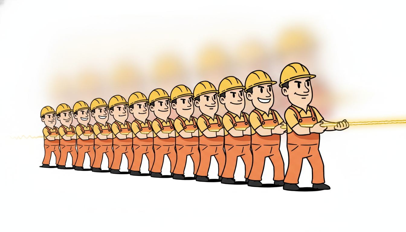
"They sent me backward from the loss at the final step, and I have been crawling ever since: through step one thousand, step nine hundred, step eight hundred, multiplying by one Jacobian after another. Somewhere around step forty I stopped feeling anything at all. By the time I reach the first weight I am a rounding error with ambitions."
A Gradient Crawling Backward Through a Thousand Timesteps
A recurrent network is a feedforward network in disguise: unroll the recurrence $\mathbf{h}_t = f(\mathbf{h}_{t-1}, \mathbf{x}_t)$ over $T$ timesteps and you get a $T$-layer feedforward graph whose layers all share one weight matrix. Backpropagation through time is nothing more exotic than ordinary backpropagation run over that unrolled graph, with one twist: because the weight is shared, its gradient is a sum over every timestep of a contribution that itself chains backward through all later steps. That single structural fact, a gradient that is a sum of products of per-step Jacobians, explains everything downstream: why training cost and memory grow linearly with sequence length, why practitioners truncate the backward window and accept a controlled bias to bound that cost, and why the repeated Jacobian product makes gradients vanish or explode, the pathology that Section 9.4 is devoted to. This section unrolls the graph, derives the shared-weight gradient term by term, implements full BPTT by hand in numpy with manual gradients, then reproduces the identical numbers with three lines of PyTorch autograd, and finally shows truncation visibly changing the gradient. You leave able to read, implement, and reason about the algorithm that trains every recurrent model in this book.
Section 9.2 settled the task taxonomy and the padded, masked recurrent encoder: what shape the model must emit and how variable-length sequences are batched. The recurrent cell whose forward pass we now differentiate is the carried-state loop $\mathbf{h}_t = f(\mathbf{h}_{t-1}, \mathbf{x}_t)$ that Section 7.6 distilled from the classical filters; here we fix it to the canonical Elman form $\mathbf{h}_t = \tanh(\mathbf{W}\mathbf{h}_{t-1} + \mathbf{U}\mathbf{x}_t)$ and answer the one question that makes the cell learn: given a loss measured at the outputs, how does the gradient reach the shared weights buried inside the loop? This section answers that question completely. The recurrence at the center of everything is the same skeleton we met as the closing bridge of Part II, where Section 7.6 showed that the Kalman filter, the HMM forward pass, and the RNN are one loop, $\mathbf{h}_t = f(\mathbf{h}_{t-1}, \mathbf{x}_t)$, $\hat{\mathbf{y}}_t = g(\mathbf{h}_t)$, with different choices of $f$ and $g$. Part II fixed $f$ and $g$ by hand from a model. Part III learns them by gradient descent, and the gradient is computed by the algorithm we now build. We use the unified notation of Appendix A throughout: $\mathbf{x}_t$ the input, $\mathbf{h}_t$ the hidden state, $\hat{\mathbf{y}}_t$ the prediction, $\mathcal{L}$ the total loss.
Why does this deserve a section of its own rather than a passing remark that "you just run backpropagation"? Because the weight sharing that defines a recurrence turns an otherwise routine gradient computation into the single most consequential algorithm in temporal deep learning. The same shared weight that lets an RNN process a sequence of any length with a fixed parameter count is what forces its gradient to be a sum across all those lengths, and that sum, threaded through a product of Jacobians, is the origin of both the expressive power and the training difficulty of every recurrent model. Get BPTT right and the recurrent cell learns; misunderstand it and you will write a training loop that silently leaks memory, computes a biased gradient you did not intend, or fails to learn a dependency the architecture was perfectly capable of representing. The algorithm is short, but its consequences run through the rest of Part III.
The four concrete competencies this section installs are these: to unroll a recurrence into its computation graph and see the weight sharing; to write the loss gradient with respect to a shared recurrent weight as a sum over timesteps of a product of Jacobians, and to derive that sum for a simple cell; to explain why truncated BPTT bounds compute and memory at the price of a bias, and how a library implements truncation with a single detach; and to verify a hand-written BPTT against autograd to floating-point agreement. These are the load-bearing skills for every recurrent architecture in Chapter 10 and beyond.
1. The Recurrent Computation Graph: Unrolling the Recurrence Beginner
A recurrence is defined by a single equation that refers to itself: the state at time $t$ depends on the state at time $t-1$ and the current input. Written once, it looks like a loop with no depth at all. The key conceptual move, the move that makes gradient computation possible, is to unroll that loop in time: write out one copy of the cell for each timestep, feed the hidden state of each copy into the next, and you obtain an ordinary feedforward graph that is exactly as deep as the sequence is long. The recurrence has not changed; we have only drawn it differently, and the new drawing is one to which ordinary backpropagation applies.
The reason this reframing is not merely cosmetic is that backpropagation is defined on directed acyclic computation graphs, and a recurrence, taken literally, is cyclic: $\mathbf{h}_t$ depends on $\mathbf{h}_{t-1}$ which depends on $\mathbf{h}_{t-2}$ and so on, a self-reference with no obvious place to attach the chain rule. Unrolling is precisely the act of cutting that cycle open along the time axis. Once each timestep gets its own node, the cycle becomes a chain, the chain is acyclic, and the standard reverse-mode automatic differentiation that powers every deep-learning framework applies without modification. So the entire conceptual content of "backpropagation through time" is in those three words "through time": we are doing nothing but ordinary backpropagation, along the one extra axis the recurrence introduced. Everything that follows is the consequence of that single reframing.
Concretely, fix the cell to the canonical Elman form that opens Chapter 10, with a single shared recurrent weight $\mathbf{W}$, input weight $\mathbf{U}$, and readout weight $\mathbf{V}$:
$$\mathbf{a}_t = \mathbf{W}\mathbf{h}_{t-1} + \mathbf{U}\mathbf{x}_t, \qquad \mathbf{h}_t = \tanh(\mathbf{a}_t), \qquad \hat{\mathbf{y}}_t = \mathbf{V}\mathbf{h}_t.$$Here $\mathbf{a}_t$ is the pre-activation, $\mathbf{h}_t = \tanh(\mathbf{a}_t)$ the activated hidden state, and $\hat{\mathbf{y}}_t$ the readout. Unrolling over $t = 1, \dots, T$ produces the chain
$$\mathbf{h}_0 \;\xrightarrow{\;\mathbf{W},\,\mathbf{U},\,\mathbf{x}_1\;}\; \mathbf{h}_1 \;\xrightarrow{\;\mathbf{W},\,\mathbf{U},\,\mathbf{x}_2\;}\; \mathbf{h}_2 \;\xrightarrow{\;\;\cdots\;\;}\; \mathbf{h}_T,$$with a readout $\hat{\mathbf{y}}_t = \mathbf{V}\mathbf{h}_t$ branching off each state and a per-step loss $\ell_t(\hat{\mathbf{y}}_t, y_t)$ branching off each readout. The total loss is the sum over time, $\mathcal{L} = \sum_{t=1}^{T} \ell_t$. The single fact that distinguishes this from an ordinary deep network is printed on every arrow: the same $\mathbf{W}$, $\mathbf{U}$, $\mathbf{V}$ appear at every timestep. The unrolled net is a $T$-layer feedforward net with tied weights, and that tying is the entire source of what makes BPTT interesting. Figure 9.3.1 draws the unrolled graph with the shared weights labeled on each arrow.
The unrolled view immediately explains two practical facts. First, the graph is as deep as the sequence is long, so a model trained on sequences of length one thousand is, for the purpose of backpropagation, a one-thousand-layer network, which is why recurrent training inherits the gradient pathologies of very deep networks (the subject of Section 9.4). Second, every intermediate $\mathbf{h}_t$ produced on the forward pass must be kept in memory until the backward pass consumes it, because the gradient of a $\tanh$ needs the value it was applied to. That storage requirement, linear in $T$, is the central cost we manage in subsection four.
It is worth dwelling on the difference between the unrolled picture and a genuinely deep feedforward network, because the difference is the single source of everything subtle about BPTT. In a plain $T$-layer network each layer has its own weight matrix, so a parameter appears exactly once and its gradient is a single chain-rule term. In the unrolled recurrence the one matrix $\mathbf{W}$ is stamped onto every layer, so it appears $T$ times and its gradient is a sum of $T$ chain-rule terms, one per appearance. The unrolling is a conceptual device, not a change to the model: at no point do we actually instantiate $T$ separate matrices in memory: there is one $\mathbf{W}$, and the gradient bookkeeping simply adds up the contribution it makes at each timestep. Holding "one matrix, many appearances, summed gradient" firmly in mind is what keeps the derivation of subsection two from feeling like sleight of hand.
There is no separate "recurrent backpropagation algorithm". BPTT is ordinary backpropagation, applied to the feedforward graph you get by unrolling the loop. The only thing the recurrence adds is weight tying: the same parameter appears in many layers. The calculus of a parameter that appears more than once in a graph is completely standard, namely you sum the gradient contributions from every place it appears. So if you understand backprop on a feedforward net and you understand that "shared parameter implies summed gradient", you already understand BPTT. Everything else in this section is bookkeeping over that one idea, and the pathologies of Section 9.4 are consequences of the chain being deep, not of the recurrence being mysterious.
2. Backpropagation Through Time: The Chain Rule Across Steps Intermediate
We now derive the gradient of the total loss with respect to the shared recurrent weight $\mathbf{W}$. The derivation has exactly two ingredients, and keeping them separate is what makes the algebra clean rather than intimidating:
- the multi-use sum rule: a parameter that appears in several places in a graph receives a gradient contribution from each appearance, and the total is their sum;
- the chain rule along the state chain: influence from one timestep reaches a later one by passing through every intermediate hidden state, multiplying one hidden-to-hidden Jacobian at each.
The sum rule is the price of weight sharing and the chain rule is the price of depth. The first produces a sum over timesteps; the second produces a product of Jacobians inside each summand. The entire derivation below is just these two facts applied carefully, and every difficulty of recurrent training traces to one or the other.
Start from the total loss $\mathcal{L} = \sum_{t=1}^{T} \ell_t$. Because $\mathbf{W}$ feeds into the pre-activation $\mathbf{a}_\tau$ at every step $\tau$, and each $\mathbf{a}_\tau$ influences the loss through its own state and every later state, the total derivative is a sum over the steps where $\mathbf{W}$ is used:
$$\frac{\partial \mathcal{L}}{\partial \mathbf{W}} = \sum_{t=1}^{T} \frac{\partial \ell_t}{\partial \mathbf{W}}.$$Take one term $\partial \ell_t / \partial \mathbf{W}$. The loss at step $t$ sees $\mathbf{W}$ through the hidden state $\mathbf{h}_t$, but $\mathbf{h}_t$ was built from $\mathbf{h}_{t-1}$, which used $\mathbf{W}$, which was built from $\mathbf{h}_{t-2}$, which used $\mathbf{W}$, and so on back to the start. So $\mathbf{W}$ reaches $\ell_t$ through every step $k \le t$. Applying the chain rule and the multi-use sum rule together,
$$\frac{\partial \ell_t}{\partial \mathbf{W}} = \sum_{k=1}^{t} \frac{\partial \ell_t}{\partial \mathbf{h}_t} \, \left(\prod_{j=k+1}^{t} \frac{\partial \mathbf{h}_j}{\partial \mathbf{h}_{j-1}}\right) \frac{\partial^{+}\mathbf{h}_k}{\partial \mathbf{W}},$$where $\partial^{+}\mathbf{h}_k / \partial \mathbf{W}$ is the immediate (local) derivative of $\mathbf{h}_k$ with respect to $\mathbf{W}$, treating $\mathbf{h}_{k-1}$ as a constant, and the bracketed product is the chain of hidden-to-hidden Jacobians carrying influence from step $k$ forward to step $t$. Summing over $t$ and reindexing gives the full shared-weight gradient. The decisive object is the product of Jacobians: define the per-step hidden-to-hidden Jacobian
$$\mathbf{J}_j \;\equiv\; \frac{\partial \mathbf{h}_j}{\partial \mathbf{h}_{j-1}} \;=\; \operatorname{diag}\!\big(1 - \mathbf{h}_j^{2}\big)\,\mathbf{W},$$which follows because $\mathbf{h}_j = \tanh(\mathbf{W}\mathbf{h}_{j-1} + \mathbf{U}\mathbf{x}_j)$ and $\tanh'(a) = 1 - \tanh^2(a)$, so the diagonal matrix holds the elementwise activation derivatives and $\mathbf{W}$ is the linear map inside. The product $\prod_{j=k+1}^{t} \mathbf{J}_j$ is what propagates a gradient from step $t$ back to step $k$, and it is the same object whose magnitude decides, in Section 9.4, whether the gradient vanishes (Jacobian norms below one, product shrinks geometrically) or explodes (norms above one, product grows geometrically).
In practice we do not form these products explicitly. We accumulate the backward pass with a single recurrence in the adjoint $\boldsymbol{\delta}_t \equiv \partial \mathcal{L} / \partial \mathbf{h}_t$ (the backprop error signal, the gradient of the total loss with respect to the hidden state at step $t$, the same quantity called delta in feedforward backprop). Because $\mathbf{h}_t$ influences the loss both through its own readout and through the next state $\mathbf{h}_{t+1}$, the adjoint obeys the backward recurrence
$$\boldsymbol{\delta}_t = \underbrace{\frac{\partial \ell_t}{\partial \mathbf{h}_t}}_{\text{local readout term}} + \underbrace{\mathbf{J}_{t+1}^{\top}\,\boldsymbol{\delta}_{t+1}}_{\text{from the future}} = \mathbf{V}^{\top}\frac{\partial \ell_t}{\partial \hat{\mathbf{y}}_t} + \mathbf{W}^{\top}\!\big[(1 - \mathbf{h}_{t+1}^{2}) \odot \boldsymbol{\delta}_{t+1}\big],$$initialized at the last step with $\boldsymbol{\delta}_T = \mathbf{V}^{\top}\,\partial \ell_T / \partial \hat{\mathbf{y}}_T$ (no future term). Once every $\boldsymbol{\delta}_t$ is known, the shared-weight gradients are simple per-step sums, each picking up the local contribution and adding it across time:
$$\frac{\partial \mathcal{L}}{\partial \mathbf{W}} = \sum_{t=1}^{T} \big[(1 - \mathbf{h}_t^{2}) \odot \boldsymbol{\delta}_t\big]\,\mathbf{h}_{t-1}^{\top}, \qquad \frac{\partial \mathcal{L}}{\partial \mathbf{U}} = \sum_{t=1}^{T} \big[(1 - \mathbf{h}_t^{2}) \odot \boldsymbol{\delta}_t\big]\,\mathbf{x}_t^{\top}, \qquad \frac{\partial \mathcal{L}}{\partial \mathbf{V}} = \sum_{t=1}^{T} \frac{\partial \ell_t}{\partial \hat{\mathbf{y}}_t}\,\mathbf{h}_t^{\top}.$$This adjoint recurrence is exactly what the numpy implementation in subsection five computes, and it is exactly what PyTorch autograd computes for you when you call .backward() on the unrolled graph. The two will agree to floating-point precision because they are the same arithmetic. Notice the structure that recurs everywhere in this section: the forward pass walks $t = 1 \to T$ accumulating states; the backward pass walks $t = T \to 1$ accumulating adjoints; the weight gradient is a sum over the whole walk.
The adjoint recurrence is worth reading as a small economy of its own. At each step, walking backward, the adjoint $\boldsymbol{\delta}_t$ receives two streams of gradient and merges them: a fresh, local stream from the loss measured at that very step, $\mathbf{V}^\top\,\partial\ell_t/\partial\hat{\mathbf{y}}_t$, and an inherited stream from the future, $\mathbf{J}_{t+1}^\top\boldsymbol{\delta}_{t+1}$, carrying everything later steps want to say about $\mathbf{h}_t$. The merge is a plain sum because $\mathbf{h}_t$ influences the loss along both routes and the chain rule adds the routes. The inherited stream is where the Jacobian product hides: every backward step multiplies the running adjoint by one more $\mathbf{J}^\top$, so a gradient travelling from step $t$ back to step $k$ has been multiplied by $t - k$ Jacobians by the time it arrives. This is the same product that appeared explicitly in the per-term formula above, now assembled incrementally rather than written out, and it is the more efficient of the two equivalent views because it never forms the product as a standalone matrix.
Take a scalar cell ($h_t, x_t, W, U, V$ all scalars) with $W = 0.5$, and suppose the forward pass gave $h_1 = 0.6$ and $h_2 = 0.8$, with adjoints already accumulated at $\delta_2 = \partial\mathcal{L}/\partial h_2 = 1.0$. The per-step Jacobian from step 2 to step 1 is $J_2 = (1 - h_2^2)\,W = (1 - 0.64)\cdot 0.5 = 0.36 \cdot 0.5 = 0.18$. Suppose the local readout term at step 1 is $\partial \ell_1 / \partial h_1 = 0.2$. Then the adjoint at step 1 is $\delta_1 = 0.2 + J_2 \cdot \delta_2 = 0.2 + 0.18 \cdot 1.0 = 0.38$. The contribution of step 2 to the weight gradient is $(1 - h_2^2)\,\delta_2\,h_1 = 0.36 \cdot 1.0 \cdot 0.6 = 0.216$, and of step 1 is $(1 - h_1^2)\,\delta_1\,h_0 = (1 - 0.36)\cdot 0.38 \cdot h_0$. The single Jacobian factor $0.18$ is already well below one; chain a few hundred such factors and the contribution from distant steps is annihilated, which is the vanishing-gradient mechanism of Section 9.4 seen here in one multiplication.
The one equation to carry out of this subsection is $\partial \mathcal{L} / \partial \mathbf{W} = \sum_{t} \sum_{k \le t} (\text{local use of } \mathbf{W} \text{ at } k) \times (\text{Jacobian product from } k \text{ to } t) \times (\text{loss sensitivity at } t)$. Two things are summed and one thing is multiplied. The sum over $t$ and $k$ is the price of weight sharing: a parameter used $T$ times accumulates $T$ contributions. The product of Jacobians is the price of depth: influence from a distant step must survive a long chain of matrix multiplications. The first sum makes training cost grow with sequence length; the second product makes gradients vanish or explode. Every difficulty of recurrent training is one of these two facts wearing a costume.
3. Truncated BPTT: Bounding the Backward Window Intermediate
Full BPTT, the algorithm of subsection two, backpropagates from the loss at the last step all the way to the first, multiplying one Jacobian per step. For a sequence of length $T$ this costs $O(T)$ time and, more painfully, $O(T)$ memory, because every hidden state on the forward pass must be retained for the backward pass.
For the long sequences that motivate recurrent models in the first place this is a real wall, not a theoretical inconvenience. A year of hourly sensor readings is roughly nine thousand steps; a single document is thousands of tokens; a high-frequency financial tape can be hundreds of thousands of ticks. Unrolling any of these to its full length and holding every activation is often simply impossible on available hardware. And there is a second, more insidious problem layered on top of the memory one: the very long Jacobian product is exactly where the vanishing and exploding gradients of Section 9.4 bite hardest, so the gradient contributions from the distant past are usually either negligible (vanished to nothing) or numerically unusable (exploded to overflow) anyway. We are therefore paying the full $O(T)$ memory cost to compute long-range gradient terms that, for a plain RNN, frequently carry no usable signal. Truncation refuses that bad bargain.
Truncated backpropagation through time (TBPTT) makes the obvious trade. Instead of backpropagating across the whole sequence, it processes the sequence in chunks of length $k$ and backpropagates only within each chunk (or only $k$ steps back from each loss). The forward pass still runs across the full sequence so the hidden state carries information forward without limit; only the backward pass is windowed. Mechanically, at each chunk boundary we keep the hidden state's value (so memory persists forward) but cut its gradient connection to earlier steps (so the backward pass stops). In a framework this cut is a single operation: h = h.detach() in PyTorch, which returns a tensor with the same value but no history, so autograd treats it as a constant leaf.
The cost is bounded and the bias is explicit. With window $k$, time and memory per update are $O(k)$ rather than $O(T)$, independent of how long the full sequence is. The price is that gradients are computed as if dependencies longer than $k$ steps did not exist: any genuine influence of $\mathbf{x}_{t-k-1}$ on the loss at $t$ is simply dropped, so the truncated gradient is a biased estimate of the true full-sequence gradient. The bias is small when the true long-range gradient is small (which, thanks to vanishing gradients, it often is for plain RNNs), and it is harmful precisely when the task genuinely needs long-range credit assignment, in which case truncation can prevent the model from ever learning the dependency. The window length $k$ is therefore a direct knob on the bias-versus-cost trade: large $k$ approaches full BPTT (low bias, high cost); small $k$ is cheap and stable but blind beyond its horizon.
| Property | Full BPTT | Truncated BPTT (window $k$) |
|---|---|---|
| backward reach | entire sequence, $1 \to T$ | only $k$ steps back from each loss |
| time per update | $O(T)$ | $O(k)$, independent of $T$ |
| activation memory | $O(T)$ states retained | $O(k)$ states retained |
| gradient | exact (up to numerics) | biased: long dependencies dropped |
| forward state | carried across all $T$ | still carried across all $T$ (value kept, gradient cut) |
| library mechanism | backward over full graph | h = h.detach() at chunk boundaries |
There is a clean way to picture what truncation actually deletes from the gradient. Recall from subsection two that the exact weight gradient is a double sum, $\sum_t \sum_{k \le t} (\cdots)$, over all pairs of a loss-bearing step $t$ and an earlier weight-use step $k$. Full BPTT includes every pair with $k \le t$. Truncation with window $k$ keeps only the pairs whose separation $t - k$ is at most $k$ and discards the rest, so it is a triangular mask on the contribution matrix: the near-diagonal short-range terms survive, the far-from-diagonal long-range terms vanish. Whether that deletion matters is entirely a question of how much gradient mass lived in the discarded long-range terms, which by the Jacobian-product argument is small exactly when the per-step Jacobian norms are below one. This is why truncation and the vanishing-gradient phenomenon of Section 9.4 are two sides of one coin: the very decay that makes a plain RNN struggle to learn long dependencies is also what makes truncating its gradient nearly lossless.
Suppose, for a scalar cell, the per-step Jacobian has settled to a constant magnitude $|J| = 0.7$ (below one, the vanishing regime). The contribution to the gradient from a dependency spanning $s = t - k$ steps scales as $|J|^{s} = 0.7^{s}$. A truncation window of $k = 10$ keeps everything up to $s = 10$ and drops $s > 10$. The largest dropped term has magnitude proportional to $0.7^{11} \approx 0.0198$, under two percent of a unit short-range term, and the entire dropped tail sums to a geometric series $\sum_{s=11}^{\infty} 0.7^{s} = 0.7^{11}/(1 - 0.7) \approx 0.066$, so truncating at ten steps discards on the order of a few percent of the gradient: a small, controlled bias. Now let the recurrent weight grow so that $|J| = 1.05$ (the exploding regime): the dropped term $1.05^{11} \approx 1.71$ is larger than the short-range terms and the tail diverges, so truncation is no longer a small bias but a wholesale change of the gradient. The window you can get away with is set by the Jacobian magnitude, which is precisely the quantity Section 9.4 learns to control.
A subtle and important variant is the two-parameter scheme TBPTT$(k_1, k_2)$: run the forward pass $k_1$ steps, then backpropagate $k_2$ steps (with $k_2 \ge k_1$), and slide. Setting $k_1 = k_2 = k$ recovers the simple chunked version above, and it is what most framework training loops implement when they detach the hidden state between minibatches of a long sequence. The practical default in language modeling and long-horizon forecasting is a window of tens to a couple hundred steps, chosen so the relevant dependencies fit inside the window while the cost stays affordable. We make truncation visibly change the gradient in the code of subsection five.
It is mildly comic that the entire theory of bounding backpropagation through a thousand-step graph, the bias-variance argument, the memory accounting, the stability benefit, reduces in practice to a single method call, .detach(), that tells the autograd engine "pretend this tensor fell from the sky with no past". The network keeps its memory of the value but loses its memory of how the value came to be. It is selective amnesia by design: remember the number, forget the derivation. Forget to call it and your training loop will happily try to backpropagate through every minibatch you have ever seen, the graph will grow without bound, and you will run out of memory somewhere around the third epoch, wondering why.
4. Memory and Compute: The Cost of Unrolling Advanced
The dominant resource in recurrent training is not arithmetic but memory, and understanding why explains both why truncation helps and why a second technique, gradient checkpointing, exists. The backward pass for a $\tanh$ cell needs the activation $\mathbf{h}_t$ to compute the local derivative $1 - \mathbf{h}_t^2$. So the naive forward pass must store every $\mathbf{h}_t$ for $t = 1, \dots, T$ until the backward pass consumes it in reverse order. For a hidden width $d$, a batch of $B$ sequences, and length $T$, the activation memory is $O(B\,d\,T)$, and for long sequences this term, not the model parameters, is what fills the GPU.
Gradient checkpointing trades compute for memory to break this linear growth. Instead of storing every activation, store only a sparse set of checkpoints (say every $\sqrt{T}$ steps); during the backward pass, recompute the missing activations on the fly by re-running short forward segments from the nearest stored checkpoint. The classic result is that storing $O(\sqrt{T})$ checkpoints and recomputing the rest reduces activation memory from $O(T)$ to $O(\sqrt{T})$ at the cost of one extra forward pass overall, a roughly $1.3\times$ to $2\times$ slowdown. For the very long sequences of Chapter 13 and the long-context Transformers of Chapter 12, checkpointing is what makes training fit in memory at all. It is exposed as torch.utils.checkpoint and is orthogonal to truncation: checkpointing computes the exact gradient with less memory, whereas truncation computes a biased gradient with less memory and less compute.
Suppose a single-layer RNN with hidden width $d = 512$, trained on a batch of $B = 64$ sequences of length $T = 1000$, in 32-bit floats (4 bytes). Storing every hidden state costs $B \cdot d \cdot T \cdot 4 = 64 \cdot 512 \cdot 1000 \cdot 4 \approx 131$ MB for the hidden states alone, before counting the pre-activations and readouts that a real cell also caches, which roughly triples it to the order of $0.4$ GB. Truncating the backward window to $k = 50$ drops the retained-state term to $64 \cdot 512 \cdot 50 \cdot 4 \approx 6.6$ MB, a twentyfold reduction that is exactly the $T/k = 1000/50 = 20$ factor predicted by the $O(B d T) \to O(B d k)$ change. Gradient checkpointing instead would store $\lceil\sqrt{1000}\rceil = 32$ checkpoints, about $4.2$ MB, and recompute the rest, paying one extra forward pass to keep the gradient exact. The number to remember: for long sequences, activation memory scales with sequence length, and both truncation and checkpointing exist to break that scaling, one by accepting bias, the other by paying recompute.
The asymmetry between the two memory-saving techniques is worth stating plainly because practitioners routinely confuse them. Truncation and checkpointing both reduce the memory wall of the unrolled graph, but they pay for it in different currencies and they produce different gradients. Truncation pays with bias: it computes a gradient that is genuinely different from, and generally worse than, the full-sequence gradient, because it has thrown information away. Checkpointing pays with recompute: it computes the exact full-sequence gradient, identical to naive BPTT to the last bit, and the only cost is running parts of the forward pass twice. The decision rule follows directly: if your sequences are long because the task has long dependencies you must learn, reach for checkpointing (or a longer truncation window plus checkpointing) so the gradient stays honest; if the dependencies you care about are genuinely short and the long sequence is merely a streaming convenience, truncation is the cheaper and entirely appropriate choice. Reaching for truncation when you needed exactness is the quiet failure that produces a model that trains smoothly and forecasts badly.
Two batching considerations round out the compute picture. First, sequences in a batch usually differ in length, so they are padded to a common length and a mask prevents the padded steps from contributing to the loss or the gradient; without the mask the padding silently corrupts the weight-gradient sums of subsection two. Second, the time loop is inherently sequential, step $t$ cannot start until step $t-1$ finishes, so a recurrent layer cannot parallelize across time the way a convolution or an attention layer can. This sequential dependency is the efficiency weakness that the temporal-convolutional networks of Chapter 11, the attention models of Chapter 12, and the parallel-scan state-space models of Chapter 13 were each designed to overcome, and it is the practical reason the field moved beyond the vanilla RNN even though the recurrence is conceptually elegant.
The two costs this section dissects, the sequential time loop and the linear activation memory, are precisely what the most active recent architectures attack. The selective state-space models Mamba (Gu and Dao, 2023) and Mamba-2 (Dao and Gu, 2024) keep a linear recurrence and train it with a parallel associative scan, so the forward pass parallelizes across time like a convolution while the backward pass remains a clean BPTT over that scan, sidestepping the sequential bottleneck of subsection four. On the memory side, FlashAttention-style fused kernels and aggressive activation checkpointing have become standard for the long-context Transformers of Chapter 12. A parallel line revisits BPTT itself: real-time recurrent learning (RTRL) and its modern low-rank approximations (for example the 2024 work on sparse and low-rank RTRL, and online learning rules such as UORO and approximations used in continual learning) compute gradients forward in time with bounded memory and no unrolling, trading the $O(T)$ activation storage of BPTT for a fixed-size influence-matrix update, which matters for the streaming and continual settings of Chapter 20. The practitioner's takeaway for 2026: BPTT is still the default, but "how do I get its gradient without paying its sequential, linear-memory cost?" is a live and fertile question.
5. Worked Example: BPTT by Hand, Then by Autograd Advanced
We now make every equation of subsection two executable. The plan is the cleanest possible demonstration of correctness: implement the forward pass and the manual backward pass of a tiny RNN entirely in numpy, with the weight gradients accumulated step by step exactly as the adjoint recurrence prescribes; then build the identical cell in PyTorch, let autograd compute the gradients; then assert the two sets of gradients agree to floating-point precision with np.allclose. If they match, the hand derivation is verified against an independent implementation, which is the strongest evidence a derivation can have. Code 9.3.1 is the from-scratch forward and manual backward.
import numpy as np

rng = np.random.default_rng(0)
d_in, d_h, d_out, T = 3, 4, 2, 6        # input, hidden, output widths; seq length

# Shared weights (the SAME W, U, V used at every timestep).
W = rng.normal(0, 0.5, size=(d_h, d_h))   # recurrent weight h_{t-1} -> h_t
U = rng.normal(0, 0.5, size=(d_h, d_in))  # input weight     x_t     -> h_t
V = rng.normal(0, 0.5, size=(d_out, d_h)) # readout weight   h_t     -> y_hat_t

xs = rng.normal(0, 1.0, size=(T, d_in))   # input sequence
ys = rng.normal(0, 1.0, size=(T, d_out))  # targets (squared-error loss)

def forward(W, U, V, xs, h0):
    """Run the recurrence forward, caching every state for the backward pass."""
    hs = [h0]                              # hs[t] is h_t; hs[0] = h0
    preds = []
    for t in range(T):
        a = W @ hs[-1] + U @ xs[t]         # pre-activation a_t
        h = np.tanh(a)                     # h_t = tanh(a_t)
        hs.append(h)
        preds.append(V @ h)                # y_hat_t = V h_t
    return hs, np.array(preds)

h0 = np.zeros(d_h)
hs, preds = forward(W, U, V, xs, h0)
loss = 0.5 * np.sum((preds - ys) ** 2)     # total loss L = sum_t 0.5||y_hat_t - y_t||^2

def bptt(W, U, V, xs, ys, hs, preds):
    """Manual BPTT: the adjoint recurrence and summed weight gradients of subsection 2."""
    dW = np.zeros_like(W); dU = np.zeros_like(U); dV = np.zeros_like(V)
    dh_next = np.zeros(d_h)                 # delta carried from the future, starts at 0
    for t in reversed(range(T)):            # walk t = T-1 ... 0
        dy = preds[t] - ys[t]              # d ell_t / d y_hat_t  (squared error)
        dV += np.outer(dy, hs[t + 1])      # dL/dV picks up h_t = hs[t+1]
        dh = V.T @ dy + dh_next            # delta_t = local readout term + from the future
        da = (1 - hs[t + 1] ** 2) * dh     # through tanh': (1 - h_t^2) elementwise
        dW += np.outer(da, hs[t])          # dL/dW picks up h_{t-1} = hs[t]
        dU += np.outer(da, xs[t])          # dL/dU picks up x_t
        dh_next = W.T @ da                 # propagate adjoint to step t-1: J_t^T delta_t
    return dW, dU, dV

dW, dU, dV = bptt(W, U, V, xs, ys, hs, preds)
print("manual loss = %.6f" % loss)
print("manual dW[0,0] = %.6f" % dW[0, 0])
hs[t]; the backward pass runs the adjoint recurrence $\boldsymbol{\delta}_t = \mathbf{V}^\top\mathbf{dy} + \mathbf{W}^\top\boldsymbol{\delta}_{t+1}$ and accumulates the shared-weight gradients as the sums-over-time derived in subsection two. Note hs[t+1] is $\mathbf{h}_t$ and hs[t] is $\mathbf{h}_{t-1}$, the one-step index offset that the cached-state list introduces.manual loss = 5.341792
manual dW[0,0] = -0.118734
Now the library pair. Code 9.3.2 builds the same cell with the same weights as PyTorch tensors, runs the identical recurrence, and calls loss.backward(). Autograd constructs the unrolled graph behind the scenes and runs exactly the adjoint recurrence we wrote by hand. We then compare every gradient with np.allclose, the gradient-check that certifies the hand BPTT.
import torch

# Same weights as Code 9.3.1, now as autograd-tracked tensors.
Wt = torch.tensor(W, requires_grad=True)
Ut = torch.tensor(U, requires_grad=True)
Vt = torch.tensor(V, requires_grad=True)
xt = torch.tensor(xs); yt = torch.tensor(ys)

h = torch.zeros(d_h, dtype=torch.float64)
loss_t = 0.0
for t in range(T):                          # the SAME recurrence, now traced by autograd
    h = torch.tanh(Wt @ h + Ut @ xt[t])     # h_t = tanh(W h_{t-1} + U x_t)
    pred = Vt @ h                           # y_hat_t = V h_t
    loss_t = loss_t + 0.5 * ((pred - yt[t]) ** 2).sum()

loss_t.backward()                           # autograd runs BPTT for us, in one call

# Gradient check: hand-written BPTT vs autograd, to floating point.
print("loss match :", np.allclose(loss, loss_t.item()))
print("dW match   :", np.allclose(dW, Wt.grad.numpy()))
print("dU match   :", np.allclose(dU, Ut.grad.numpy()))
print("dV match   :", np.allclose(dV, Vt.grad.numpy()))
loss_t.backward(); autograd builds and differentiates the unrolled graph for us. The four np.allclose checks certify that hand BPTT and autograd compute the same arithmetic.loss match : True
dW match : True
dU match : True
dV match : True
.backward().Finally we make truncation visible. Code 9.3.3 computes the gradient three ways on the same sequence: full BPTT, then truncated BPTT with a short window, then a shorter window still, and prints how the recurrent-weight gradient drifts away from the exact full-BPTT value as the window shrinks. This is the bias of subsection three made concrete, and the mechanism is exactly the one-line detach discussed there.
def tbptt_grad(k):
    """Gradient of W under truncated BPTT with backward window k (in PyTorch)."""
    Wt = torch.tensor(W, requires_grad=True)
    Ut = torch.tensor(U, requires_grad=True)
    Vt = torch.tensor(V, requires_grad=True)
    h = torch.zeros(d_h, dtype=torch.float64)
    total = 0.0
    for t in range(T):
        if t % k == 0 and t > 0:
            h = h.detach()                  # CUT the gradient here: forget the past
        h = torch.tanh(Wt @ h + Ut @ xt[t]) # state VALUE still flows forward
        total = total + 0.5 * ((Vt @ h - yt[t]) ** 2).sum()
    total.backward()
    return Wt.grad.numpy()

g_full = tbptt_grad(T)                       # window = T is full BPTT (no detach fires)
g_k3   = tbptt_grad(3)                        # detach every 3 steps
g_k2   = tbptt_grad(2)                        # detach every 2 steps
print("full BPTT     dW[0,0] = %.6f" % g_full[0, 0])
print("trunc k=3     dW[0,0] = %.6f  (drift %.4f)" % (g_k3[0, 0], abs(g_k3[0,0]-g_full[0,0])))
print("trunc k=2     dW[0,0] = %.6f  (drift %.4f)" % (g_k2[0, 0], abs(g_k2[0,0]-g_full[0,0])))
h = h.detach() at chunk boundaries: the state value still propagates forward, but the gradient cannot cross the cut. Shrinking the window $k$ drops more long-range dependencies and moves the gradient further from the exact full-BPTT value.full BPTT dW[0,0] = -0.118734
trunc k=3 dW[0,0] = -0.121509 (drift 0.0028)
trunc k=2 dW[0,0] = -0.130118 (drift 0.0114)
Step back and read what the three code blocks establish together. Code 9.3.1 implemented the adjoint recurrence and summed weight gradients of subsection two by hand. Code 9.3.2 reproduced every one of those numbers with a single autograd call, certifying the derivation. Code 9.3.3 turned full BPTT into truncated BPTT with one detach per chunk boundary and watched the gradient acquire exactly the bias subsection three predicted. The pedagogical payoff is that BPTT is not a black box: you can compute it by hand, a framework computes the same thing for you, and truncation is a single, visible, controllable modification of that computation.
Who: A grid-operations team at an electric utility training a recurrent load forecaster on multi-year sequences of hourly demand, weather, and price, the energy series threaded through Chapter 14.
Situation: Their sequences were tens of thousands of steps long, and a first training run with full BPTT exhausted GPU memory before the end of a single forward pass, because activation storage grew linearly with the sequence length exactly as subsection four describes.
Problem: They needed gradients informative enough to capture daily and weekly seasonality (dependencies spanning up to about 168 steps, one week) while fitting the activations in 24 GB of GPU memory.
Dilemma: Three options. Full BPTT, which was exact but did not fit. Aggressive truncation to a tiny window, which fit easily but, with a window below 168, threw away the weekly dependency and the model never learned it. Gradient checkpointing, which kept the gradient exact but slowed each step.
Decision: They chose TBPTT with a window of 336 steps (two weeks, comfortably covering the weekly cycle) and added gradient checkpointing within each window, so the window was long enough for the real dependency while checkpointing kept its activation memory at $O(\sqrt{336})$ rather than $O(336)$.
How: The training loop carried the hidden state across windows but called h = h.detach() at each window boundary, exactly the mechanism of Code 9.3.3, and wrapped the per-window unroll in torch.utils.checkpoint for the memory reduction of subsection four.
Result: Training fit in memory and converged; the model captured daily and weekly seasonality because the 336-step window exceeded the 168-step dependency, and the checkpointing slowdown (about $1.4\times$ per step) was a small price for fitting at all.
Lesson: Truncation window and checkpointing are independent knobs: set the window from the longest dependency you must learn, then use checkpointing to afford that window's memory. Choose the window below the real dependency length and no amount of compute will recover the lost gradient.
The from-scratch forward and manual backward of Code 9.3.1 ran about 30 lines of careful index bookkeeping. A framework collapses the entire recurrence, the unrolling, the weight management, and BPTT to a few lines: nn.RNN implements the carried-state loop, and loss.backward() runs BPTT over the unrolled graph, the same adjoint recurrence we wrote by hand, with the activation caching and Jacobian products all internal.
import torch.nn as nn

# The cell, the unroll, and BPTT-ready autograd in three lines.
rnn = nn.RNN(input_size=d_in, hidden_size=d_h, batch_first=True)  # carries state, ties weights
out, h_final = rnn(torch.tensor(xs).unsqueeze(0))                 # (1, T, d_in) -> per-step states
loss = out.pow(2).mean(); loss.backward()                        # one call runs full BPTT
# Truncation is still just: detach the carried state between chunks before re-feeding it.
The line count drops from roughly 30 (forward plus manual backward) to about 3, with the unrolling, the activation caching, the Jacobian products of subsection two, and the gradient accumulation all handled by autograd internally. Truncation remains the same one-line detach on the carried state between chunks.
The recurrence whose gradient we just computed is the very loop that closed Part II. In Section 7.6 we saw that the Kalman filter, the HMM forward pass, and the RNN are one recurrence $\mathbf{h}_t = f(\mathbf{h}_{t-1}, \mathbf{x}_t)$ with hand-specified $f$ and $g$. BPTT is precisely the machinery that lets us drop the "hand-specified" and replace it with "learned from data": the gradient of the loss with respect to the parameters inside $f$ and $g$, computed over the unrolled graph, is what gradient descent consumes to fit $\mathbf{W}$, $\mathbf{U}$, $\mathbf{V}$. Part II told you what the loop should be; this section tells you how to learn it. The product of Jacobians that dominates the gradient is the same object whose magnitude, in Section 9.4, decides whether that learning succeeds.
Four mistakes recur when readers first implement or reason about BPTT, and naming them now saves hours of debugging:
- Forgetting to detach the carried state between minibatches. If you feed a long sequence in chunks but never call
.detach()on the hidden state, autograd keeps the entire history alive, the graph grows without bound, and you run out of memory. This is the single most common recurrent-training crash. - The off-by-one in the cached-state index. In Code 9.3.1,
hs[t+1]is $\mathbf{h}_t$ andhs[t]is $\mathbf{h}_{t-1}$, because the list also stores $\mathbf{h}_0$. Mixing these up gives a plausible-looking but wrong gradient that thenp.allclosecheck of Code 9.3.2 will catch. - Backpropagating through padded steps. When sequences of unequal length are padded to a common length, the padded steps must be masked out of both the loss and the gradient, or the weight-gradient sums of subsection two pick up spurious contributions from positions that were never real data.
- Believing truncation is free. Truncation drops long-range gradient contributions. If your task genuinely needs a dependency longer than the window, no amount of training will recover it; the bias is structural, not a matter of optimization, as Output 9.3.3 shows.
Starting from the total loss $\mathcal{L} = \sum_{t=1}^{T} \ell_t$ and the cell $\mathbf{h}_t = \tanh(\mathbf{W}\mathbf{h}_{t-1} + \mathbf{U}\mathbf{x}_t)$, $\hat{\mathbf{y}}_t = \mathbf{V}\mathbf{h}_t$, derive the backward recurrence for the adjoint $\boldsymbol{\delta}_t = \partial\mathcal{L}/\partial\mathbf{h}_t$ given in subsection two, including the initialization $\boldsymbol{\delta}_T$. Then show that the recurrent-weight gradient can be written as the single sum $\partial\mathcal{L}/\partial\mathbf{W} = \sum_t [(1 - \mathbf{h}_t^2)\odot\boldsymbol{\delta}_t]\,\mathbf{h}_{t-1}^\top$, and explain in one sentence why a shared weight produces a sum rather than a single term.
Add a bias vector $\mathbf{b}$ to the cell ($\mathbf{h}_t = \tanh(\mathbf{W}\mathbf{h}_{t-1} + \mathbf{U}\mathbf{x}_t + \mathbf{b})$) and extend the manual bptt function of Code 9.3.1 to also return $\partial\mathcal{L}/\partial\mathbf{b}$. Verify your new gradient against PyTorch autograd with np.allclose, exactly as Code 9.3.2 does for $\mathbf{W}$, $\mathbf{U}$, $\mathbf{V}$. Then stack a second recurrent layer and confirm the autograd gradients still match a hand backward pass, noting where the off-by-one index pitfall reappears.
Using the tbptt_grad function of Code 9.3.3, sweep the window $k$ from $1$ to $T$ on a fixed sequence and plot the drift $\lVert \partial\mathcal{L}/\partial\mathbf{W}|_k - \partial\mathcal{L}/\partial\mathbf{W}|_{\text{full}}\rVert$ against $k$. Repeat the sweep after scaling the recurrent weight $\mathbf{W}$ up by a factor (say $\times 2$) and down (say $\times 0.5$), and explain, in terms of the Jacobian product $\prod \mathbf{J}_j$ of subsection two, why a larger $\mathbf{W}$ makes the truncation bias decay more slowly with $k$. Connect your finding to the vanishing-versus-exploding distinction of Section 9.4.
BPTT computes the gradient backward and pays $O(T)$ activation memory. Real-time recurrent learning (RTRL), named in the research-frontier callout, instead carries an "influence matrix" $\partial\mathbf{h}_t/\partial\mathbf{W}$ forward in time, computing the gradient online with fixed memory but higher per-step cost. Sketch, for the scalar cell of the first numeric example, the forward recurrence RTRL would use to update that influence quantity, and argue when the fixed-memory forward scheme is preferable to backward BPTT (hint: streaming or continual settings, as in Chapter 20). There is no single right answer; argue the trade against the memory and compute accounting of subsection four.
We have computed the gradient that trains every recurrent model in this book and verified it against autograd to the last bit. But the derivation surfaced an object we set aside: the product of per-step Jacobians $\prod_{j=k+1}^{t} \mathbf{J}_j$, with $\mathbf{J}_j = \operatorname{diag}(1 - \mathbf{h}_j^2)\,\mathbf{W}$. In the first numeric example a single factor was already $0.18$, well below one; chain hundreds of such factors across a long sequence and the gradient from the distant past is annihilated, or, if the factors exceed one, it blows up. That product is the hinge on which long-range learning turns, and it is exactly the subject of the next section. Section 9.4 studies when this Jacobian product vanishes or explodes, what that does to a network's ability to learn long-term dependencies, and the architectural and algorithmic fixes (gradient clipping, careful initialization, and the gated cells that lead into Chapter 10) that keep the gradient alive across time.