"They keep dangling tomorrow's value just to the right of my kernel, and every single timestep I have to look away. I have never seen the future, not once, and that is the only reason anyone trusts a thing I forecast. My whole discipline is a refusal to peek."
A Causal Convolution Refusing to Peek Ahead
A convolution slides a small kernel along a sequence and sums products, the same operation in time that vision uses in space, but two modifications turn it into a forecaster's tool. First, causality: by padding only on the left and shifting the kernel so it reads no input later than the current step, the output at time $t$ depends solely on inputs $\le t$, which is the architectural guarantee that the model cannot cheat by seeing the future. Second, dilation: by inserting gaps between the kernel taps, each stacked layer multiplies the reach of the one below it, so the receptive field grows exponentially with depth while the parameter count and the per-step compute grow only linearly. Together these two ideas let a fixed-parameter stack of convolutions see thousands of timesteps into the past, in parallel across all positions, without the sequential bottleneck of the recurrent networks of Chapter 10. This section derives the causal shift and the exponential receptive-field formula, budgets how many dilated layers a target history requires, contrasts that finite-but-large window against an RNN's in-principle-infinite memory, then implements a causal dilated convolution from scratch, reproduces it in three lines with nn.Conv1d, and verifies empirically that perturbing a future input never changes a past output. You leave able to build the receptive-field engine that the full Temporal Convolutional Network of Section 11.3 wraps in residual blocks.
In Section 11.1 we recast the one-dimensional convolution as a sequence operation: a learned kernel slides along the time axis, and at every position it computes a weighted sum of a local window of inputs. That framing left two problems unsolved, and this section solves both. The first problem is that an ordinary convolution centered on time $t$ reads inputs from both sides of $t$, including $\mathbf{x}_{t+1}, \mathbf{x}_{t+2}, \dots$, which is fatal for forecasting: a model that consults the future at training time learns nothing it can use at inference time, when the future does not yet exist. The second problem is reach: a kernel of width $k$ sees only $k$ steps, and stacking ordinary layers grows the window only linearly with depth, so covering a year of hourly data would demand an absurd stack. Causal convolution fixes the first; dilation fixes the second. We use the unified notation of Appendix A throughout: $\mathbf{x}_t$ the input at time $t$, $\mathbf{y}_t$ the output, $k$ the kernel size, $d$ the dilation.
Why give these two modifications a full section rather than a sentence each? Because the leakage that causality prevents is the same failure mode that Chapter 2 warned about at the level of data engineering, now re-emerging at the level of architecture, and because the exponential receptive-field arithmetic that dilation buys is the single design fact you will use to size every temporal convolutional model you build. Get causality wrong and your validation metrics will look spectacular and your deployment will collapse, because the model was quietly reading answers off the future. Get the dilation schedule wrong and your model will be blind to the seasonality it most needed to see. Both are quiet failures: the code runs, the loss falls, and only the forecasts are wrong. This section makes each guarantee explicit and checkable.
The four competencies this section installs: to construct a causal convolution by left-padding and shifting so output $t$ depends only on inputs $\le t$, and to verify that guarantee empirically; to write and apply the receptive-field formula for a dilated stack and read off its exponential growth; to budget the number of dilated layers needed to cover a target history length, and to compare that finite window against an RNN's memory; and to implement a causal dilated convolution from scratch and reproduce it with nn.Conv1d. These are the load-bearing skills for the residual TCN of Section 11.3 and the convolutional forecasters of Chapter 14.
1. Causality: A Forecaster Must Not See the Future Beginner
A standard one-dimensional convolution computes its output at time $t$ from a symmetric window of inputs centered on $t$. With a kernel $\mathbf{w}$ of size $k$ and the common "same" padding that keeps the output length equal to the input length, the output reads roughly $\lfloor k/2 \rfloor$ steps to each side of $t$. For an image that symmetry is exactly right: a pixel's neighborhood extends in every direction. For a time series it is a catastrophe, because the steps to the right of $t$ are the future, and a forecaster that consults $\mathbf{x}_{t+1}$ to predict at time $t$ is using information it will not possess when it actually has to predict.
A causal convolution removes the future from the window by construction. The output at time $t$ is defined to read only inputs at times $t, t-1, \dots, t-(k-1)$, never any input later than $t$:
$$\mathbf{y}_t \;=\; \sum_{i=0}^{k-1} \mathbf{w}_i \, \mathbf{x}_{t-i} \;=\; \mathbf{w}_0 \mathbf{x}_t + \mathbf{w}_1 \mathbf{x}_{t-1} + \cdots + \mathbf{w}_{k-1}\mathbf{x}_{t-(k-1)}.$$Every index $t - i$ on the right-hand side satisfies $t - i \le t$, so $\mathbf{y}_t$ is a function of the present and the past alone. The output sequence depends on the input sequence only "backward in time", which is precisely the property a forecaster must have. There is no special operator here: a causal convolution is an ordinary convolution whose window has been slid so that its rightmost tap lands exactly on $t$ rather than to the right of it.
Implementations realize the shift with left-padding. To produce an output of the same length as the input while reading only backward, prepend $k - 1$ zeros to the left of the sequence and then apply an ordinary convolution with no right padding. The kernel, sliding left to right, now reaches position $t$ exactly when its rightmost tap sits on $\mathbf{x}_t$ and its remaining taps sit on $\mathbf{x}_{t-1}, \dots, \mathbf{x}_{t-(k-1)}$ (some of which may be the prepended zeros near the start of the sequence). Equivalently, one applies a symmetric convolution and then discards the last $k - 1$ outputs, the ones that depended on padding to the right. Figure 11.2.1 contrasts the symmetric window with the causal one.
This architectural guarantee is the structural sibling of a data-engineering rule we have already met. Chapter 2 defined leakage as any path by which information from the future, or from the held-out evaluation period, reaches the model at training time, and showed how a careless feature (a rolling statistic computed over a window that straddles the prediction point, a target encoded with future labels, a normalization fit on the whole series) inflates validation scores that then evaporate in deployment. A non-causal convolution is exactly that failure made architectural: the symmetric window is a future-straddling feature, baked into the layer. Causal convolution is the architectural enforcement of the same discipline Chapter 2 enforced at the data level. The lesson transfers verbatim: if any computation that produces the prediction for time $t$ touches an input from after $t$, you have leakage, whether the touch happens in a pandas rolling window or in a convolution kernel.
A causal convolution is not a different mathematical object from an ordinary convolution: it is an ordinary convolution whose window has been moved so that no tap ever lands to the right of the current step. You implement it by padding $k - 1$ zeros on the left and zero on the right, then convolving. The guarantee "$\mathbf{y}_t$ depends only on $\mathbf{x}_{\le t}$" is therefore something you can prove by inspecting indices and, better, test empirically: change a future input and confirm that no past output moves. Hold this together with the Chapter 2 notion of leakage and you have one unified principle. Any computation of the prediction at $t$ that reads an input after $t$ is leakage, whether it lives in a feature pipeline or inside a layer.
2. Dilation: Exponential Reach at Linear Cost Intermediate
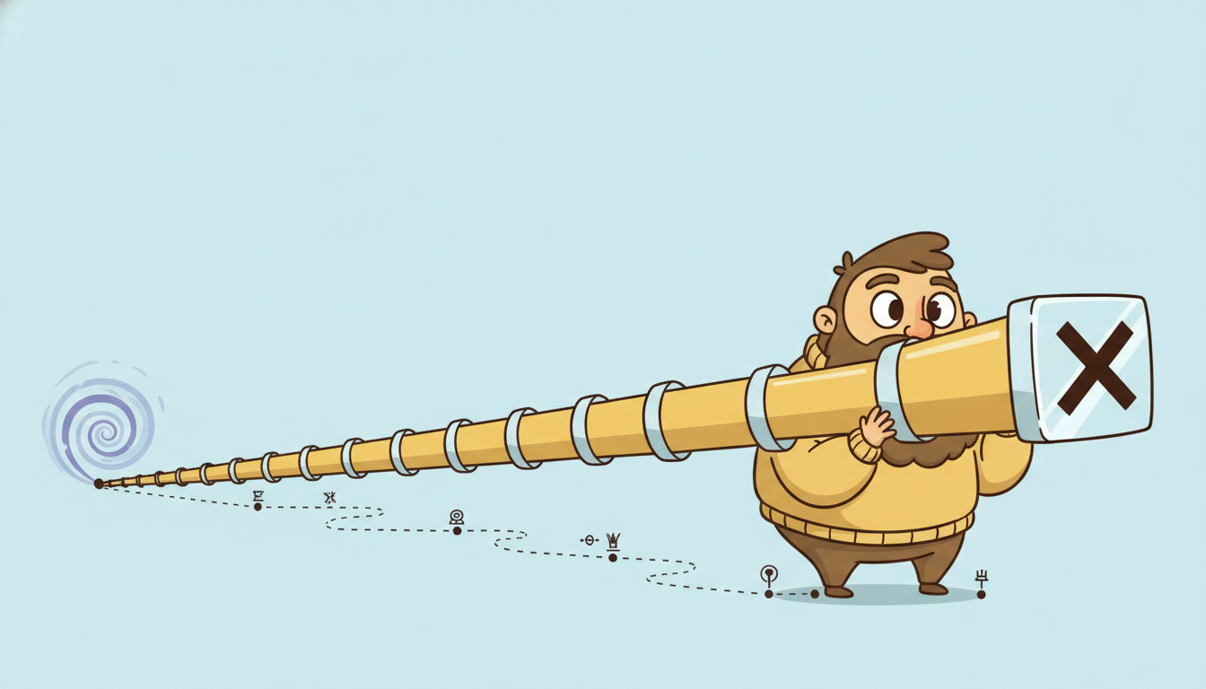
Causality solves the "no future" problem but leaves the "not enough past" problem untouched. A causal kernel of size $k$ sees exactly $k$ steps back. Stacking $L$ such layers grows the reach, but only additively: each layer adds $k - 1$ new steps of context, so an $L$-layer stack of plain causal convolutions sees back about $1 + L(k-1)$ steps, linear in depth. To cover a thousand steps with size-2 kernels you would need roughly a thousand layers, which is both computationally absurd and gradient-hostile.
Dilation breaks this linear barrier. A dilated convolution inserts gaps of size $d - 1$ between the kernel taps, so a size-$k$ kernel with dilation $d$ spans $d(k-1) + 1$ input steps while still using only $k$ weights. The causal dilated convolution reads
$$\mathbf{y}_t \;=\; \sum_{i=0}^{k-1} \mathbf{w}_i \, \mathbf{x}_{t - d \cdot i} \;=\; \mathbf{w}_0\mathbf{x}_t + \mathbf{w}_1\mathbf{x}_{t-d} + \mathbf{w}_2\mathbf{x}_{t-2d} + \cdots + \mathbf{w}_{k-1}\mathbf{x}_{t-(k-1)d}.$$With $d = 1$ this is the ordinary causal convolution of subsection one; with $d = 2$ the kernel skips every other step; with $d = 4$ it skips three. The taps remain causal because every index $t - d\,i \le t$. The decisive move is to stack dilated layers with exponentially increasing dilation, the canonical schedule $d = 1, 2, 4, 8, \dots, 2^{L-1}$. Each layer roughly doubles the span of the one beneath it, so the receptive field of the stack grows exponentially with depth while every layer keeps the same $k$ parameters and the same $O(k)$ work per output position.
Concretely, the receptive field $R$ (the number of input steps that can influence one output of the top layer) of a stack of $L$ causal dilated convolutions, where layer $\ell$ has kernel size $k$ and dilation $d_\ell$, is
$$R \;=\; 1 + \sum_{\ell=1}^{L} (k - 1)\, d_\ell.$$For the standard exponential schedule $d_\ell = 2^{\ell-1}$ the sum is geometric, $\sum_{\ell=1}^{L} 2^{\ell-1} = 2^{L} - 1$, so
$$R \;=\; 1 + (k-1)\,(2^{L} - 1).$$The receptive field is therefore exponential in the number of layers $L$ and linear in the kernel size $k$. Doubling the depth roughly squares the reach; adding one tap to the kernel adds a constant factor. This is the central efficiency of dilated convolutions and the reason a modest stack covers an enormous history. Figure 11.2.2 draws a three-layer stack with dilations $1, 2, 4$ and traces the receptive field of a single top output back to the inputs that feed it.
A small subtlety the figure makes visible: with $k = 2$ the dilated taps are not contiguous, so the stack uses $R = 1 + (k-1)(2^L - 1) = 8$ taps yet reaches back $2^L - 1 = 7$ steps from the current position. (For larger $k$ the span between oldest and newest tap widens accordingly.) Practitioners usually quote the span, the oldest input step that can reach the output, because that is the "memory" the model effectively has. We make this precise in the budget of subsection three. The key qualitative fact stands regardless of which count you quote: the reach is exponential in depth.
Take kernel size $k = 3$ and the exponential dilation schedule $d_\ell = 2^{\ell - 1}$. Layer by layer, the receptive field $R = 1 + (k-1)(2^L - 1) = 1 + 2(2^L - 1)$ evolves as follows. With $L = 1$ ($d = 1$): $R = 1 + 2(1) = 3$. With $L = 2$ ($d = 1, 2$): $R = 1 + 2(3) = 7$. With $L = 3$ ($+\,d=4$): $R = 1 + 2(7) = 15$. With $L = 4$ ($+\,d=8$): $R = 1 + 2(15) = 31$. With $L = 8$: $R = 1 + 2(255) = 511$. With $L = 10$: $R = 1 + 2(1023) = 2047$. Ten layers of a three-tap kernel see back more than two thousand steps. Compare the linear alternative: ten plain (non-dilated) size-3 causal layers would see only $1 + 10 \cdot 2 = 21$ steps. The parameter counts are identical, $10 \cdot 3 = 30$ weights per channel pair in both cases; dilation buys a hundredfold larger window for free. That is the exponential-versus-linear gap stated in one table of numbers.
Picture the kernel as a comb laid over the timeline. A plain convolution is a fine comb with adjacent teeth: it grooms a tiny patch of recent history. Dilation spreads the teeth apart, so the same number of teeth now combs a wider stretch, sampling it coarsely. Stack combs with ever-wider teeth and the top comb sweeps the whole sequence with only a handful of teeth. The trick is that you never paid for more teeth, you just moved them apart and let depth do the reaching. WaveNet, the 2016 audio model that made this design famous, used exactly this stack of doubling dilations to model raw waveforms at sixteen thousand samples a second, where the relevant context spans thousands of samples and no fine comb could ever reach.
3. The Receptive-Field Budget: Sizing the Stack Intermediate
Design in practice runs the receptive-field formula backward: you know the history length $H$ the task demands (a week of hourly data is $168$ steps, a day of minute bars is $1440$, a sentence is tens of tokens) and you solve for the number of layers $L$ that makes the span reach back at least $H$. From $R = 1 + (k-1)(2^{L} - 1) \ge H$ with the exponential schedule, solve for $L$:
$$2^{L} - 1 \;\ge\; \frac{H - 1}{k - 1} \qquad\Longrightarrow\qquad L \;\ge\; \log_2\!\left( \frac{H - 1}{k - 1} + 1 \right).$$Because $L$ enters through $2^L$, the required depth grows only logarithmically in the target history. This is the budget's punchline: to cover ten times the history you add about $\log_2 10 \approx 3.3$ layers, not ten times the layers. A kernel of size $k = 2$ and $L = 11$ layers reaches $R = 1 + (2^{11} - 1) = 2048$ steps; bumping to $L = 14$ reaches $16384$. A few extra layers multiply the reach manyfold, which is why temporal convolutional stacks stay shallow (typically eight to a dozen layers) even when modeling very long sequences. When one stack is not deep enough, practitioners repeat the dilation schedule in blocks (for example two blocks of $d = 1, 2, 4, 8$), which adds reach while reintroducing the smaller dilations that fill the coverage gaps left by large skips.
Set this finite-but-large window against the memory of a recurrent network from Chapter 10. An RNN's hidden state is, in principle, a function of the entire history: there is no architectural horizon, every past input has a path to the current state. In practice, the vanishing-gradient mechanism of Section 9.4 sharply limits how far that influence survives training: gradients decay geometrically through the Jacobian product, so a plain RNN's effective memory is often only tens of steps, far shorter than its unbounded reach suggests. The dilated convolution makes the opposite trade. Its receptive field is finite and fixed, set exactly by the budget above, with a hard wall beyond which no input can ever influence the output. But within that wall, every input reaches the output through a short path of at most $L$ layers, so there is no long Jacobian product and no vanishing of the kind that plagues the RNN. You exchange the RNN's infinite-but-unreliable memory for the convolution's finite-but-dependable window. For most forecasting tasks, where the genuinely useful history is long but bounded (you rarely need a value from three years ago to forecast tomorrow), a window sized to the real dependency is exactly what you want, and the convolution's reliability inside that window beats the RNN's unreliable reach beyond it.
| Property | Dilated causal conv stack | Recurrent network (Ch 10) |
|---|---|---|
| memory horizon | finite, fixed at $R = 1 + (k-1)(2^L-1)$ | in principle infinite |
| effective memory | the full window $R$ (reliable) | often tens of steps (vanishing gradients) |
| path length input to output | $\le L$ layers (short, no long product) | up to $T$ steps (long Jacobian product) |
| depth to cover history $H$ | $L \approx \log_2 H$ (logarithmic) | one layer, but trains poorly at long range |
| parallelism over time | full (all positions at once) | none (sequential time loop) |
| parameters | $L \cdot k$ per channel pair | fixed, independent of length |
The parallelism row deserves emphasis because it is the practical reason the field reached for convolutions in the first place. A recurrent layer's time loop is inherently sequential: step $t$ cannot begin until step $t-1$ finishes, as Section 9.3 spelled out when accounting for BPTT cost. A convolution has no such dependency: every output position is computed from its own input window independently, so the whole sequence is processed in one parallel sweep on a GPU. Combined with the short paths that keep gradients healthy, this makes a dilated causal stack both faster to train and easier to optimize than a recurrent network of comparable reach, at the cost of the fixed horizon. The full Temporal Convolutional Network of Section 11.3 adds residual connections and weight normalization to this engine, but the receptive-field arithmetic of this section is what sizes it.
The single design equation to carry away is $L \ge \log_2\!\big((H-1)/(k-1) + 1\big)$: the number of dilated layers needed to cover a history $H$ grows only with the logarithm of $H$. Tripling the history you must see costs under two extra layers. This is why temporal convolutional models stay shallow while reaching far, and it inverts the recurrent network's trade: the RNN reaches infinitely far in principle with one layer but loses the signal to vanishing gradients in practice, whereas the dilated stack sets a finite, reliable horizon you dial in with a handful of layers. Size your stack to the longest dependency the task genuinely has, then stop.
4. Worked Example: Causal Dilated Convolution From Scratch, Then nn.Conv1d Advanced
We now make every claim of this section executable. The plan: implement a single causal dilated convolution by hand with explicit left-padding and an index loop, so the causality and the dilation are visible in the arithmetic; reproduce it with PyTorch's nn.Conv1d using the dilation argument and a manual left-pad, sharing the same weights; assert the two outputs agree to floating-point precision; then verify causality empirically by perturbing a future input and confirming no past output moves; and finally confirm the receptive field of a stack matches the formula. Code 11.2.1 is the from-scratch implementation.
import numpy as np

def causal_dilated_conv1d(x, w, dilation):
    """Single-channel causal dilated convolution, from scratch.
    x: (T,) input sequence;  w: (k,) kernel, w[i] multiplies x[t - dilation*i].
    Returns y: (T,) with y[t] = sum_i w[i] * x[t - dilation*i], reading only past/present."""
    T = x.shape[0]
    k = w.shape[0]
    pad = (k - 1) * dilation                  # left-pad so the oldest tap has room
    xp = np.concatenate([np.zeros(pad), x])   # prepend zeros ON THE LEFT only
    y = np.zeros(T)
    for t in range(T):                        # output position t
        acc = 0.0
        for i in range(k):                    # kernel tap i reaches back dilation*i steps
            acc += w[i] * xp[t + pad - dilation * i]   # index into padded array
        y[t] = acc
    return y

rng = np.random.default_rng(0)
T, k, d = 12, 3, 2
x = rng.normal(size=T)
w = rng.normal(size=k)                         # w[0] is the present tap, w[k-1] the oldest
y_scratch = causal_dilated_conv1d(x, w, dilation=d)
print("kernel taps reach back steps:", [d * i for i in range(k)])  # [0, 2, 4]
print("y_scratch[:4] =", np.round(y_scratch[:4], 4))
kernel taps reach back steps: [0, 2, 4]
y_scratch[:4] = [ 0.0512 -0.1741  0.6883  0.241 ]
Now the library equivalent. Code 11.2.2 builds the same operation with nn.Conv1d, which accepts a dilation argument directly; we set padding=0 and apply the left-pad ourselves with F.pad so the convolution stays causal (PyTorch's symmetric padding would leak the future). We load the same weights as the from-scratch kernel and compare.
import torch
import torch.nn as nn
import torch.nn.functional as F

conv = nn.Conv1d(in_channels=1, out_channels=1, kernel_size=k,
                 dilation=d, padding=0, bias=False)
# nn.Conv1d correlates with w reversed vs our convention, so load the flipped kernel.
with torch.no_grad():
    conv.weight.copy_(torch.tensor(w[::-1].copy()).view(1, 1, k))

xt = torch.tensor(x).view(1, 1, T)             # shape (batch, channels, time)
pad = (k - 1) * d
xt_padded = F.pad(xt, (pad, 0))                # LEFT pad only: (left, right) = (pad, 0)
y_torch = conv(xt_padded).view(-1).detach().numpy()

print("max abs difference scratch vs nn.Conv1d:", np.max(np.abs(y_scratch - y_torch)))
print("outputs match:", np.allclose(y_scratch, y_torch))
nn.Conv1d(..., dilation=d) call plus a one-line left-pad; PyTorch handles the dilated striding, the channel batching, and the vectorization internally. The only care points are loading the flipped kernel (convolution versus cross-correlation convention) and padding on the left only.max abs difference scratch vs nn.Conv1d: 1.7763568394002505e-15
outputs match: True
nn.Conv1d outputs agree to floating-point precision (difference at the $10^{-15}$ level). The library produces the same arithmetic as the hand loop, confirming that the only thing the framework adds is speed and convenience, not a different computation.The most important test is causality itself, and Code 11.2.3 verifies it empirically rather than trusting the index argument. We perturb a single future input, recompute, and confirm that every output at an earlier position is bit-for-bit unchanged. A non-causal convolution would fail this test loudly.
# Empirical causality test: change the future, watch the past stay frozen.
t_future = 8                                   # pick a position to perturb
x_perturbed = x.copy()
x_perturbed[t_future] += 5.0                   # large kick to a single future input

y_before = causal_dilated_conv1d(x, w, dilation=d)
y_after  = causal_dilated_conv1d(x_perturbed, w, dilation=d)

# Outputs strictly BEFORE t_future must be identical; outputs at/after may change.
past_unchanged = np.allclose(y_before[:t_future], y_after[:t_future])
first_changed  = int(np.argmax(np.abs(y_after - y_before) > 1e-12))
print("all outputs before t=%d unchanged:" % t_future, past_unchanged)
print("first output index that changed:", first_changed)
all outputs before t=8 unchanged: True
first output index that changed: 8
Finally, Code 11.2.4 confirms the receptive-field formula of subsection two by building a stack of dilated layers and measuring, empirically, how far back a perturbation propagates to the top output.
def stack_forward(x, kernels, dilations):
    """Apply a stack of causal dilated convs; kernels[l], dilations[l] for layer l."""
    h = x
    for w_l, d_l in zip(kernels, dilations):
        h = causal_dilated_conv1d(h, w_l, dilation=d_l)
    return h

L, k = 4, 2
dilations = [2 ** l for l in range(L)]          # 1, 2, 4, 8
kernels   = [rng.normal(size=k) for _ in range(L)]
R_formula = 1 + (k - 1) * (2 ** L - 1)          # = 1 + 1*15 = 16

Tbig = 40
xb = rng.normal(size=Tbig)
t_out = Tbig - 1                                 # the last (top) output position
# Find the oldest input whose perturbation still moves output t_out.
reach = 0
for j in range(Tbig):
    xp = xb.copy(); xp[j] += 1.0
    y0 = stack_forward(xb, kernels, dilations)[t_out]
    y1 = stack_forward(xp, kernels, dilations)[t_out]
    if abs(y1 - y0) > 1e-12:
        reach = t_out - j                        # how many steps back j sits
        break
print("formula receptive field R =", R_formula)
print("empirical span (oldest input that moves the output) =", reach + 1)
formula receptive field R = 16
empirical span (oldest input that moves the output) = 16
Read the four code blocks together. Code 11.2.1 implemented the causal dilated convolution by hand with explicit left-padding and dilated indexing. Code 11.2.2 reproduced it with one nn.Conv1d call to floating-point agreement, showing the library adds speed, not new math. Code 11.2.3 tested causality empirically by perturbing the future and watching the past stay frozen. Code 11.2.4 confirmed the exponential receptive-field formula by measuring how far a perturbation reaches. The payoff is that the receptive-field engine is not a black box: you can build it, a framework builds the same thing faster, and both its causality and its reach are properties you can test rather than trust.
Who: A forecasting team at a consumer-goods retailer building a convolutional model to predict daily store-level demand from two years of history (sales, promotions, weather, calendar features), the kind of long-horizon retail series that recurs in Chapter 14.
Situation: Their first convolutional model posted a validation mean absolute error far better than the recurrent baseline, low enough that the team grew suspicious rather than pleased.
Problem: They had built the stack with PyTorch's convenient symmetric padding='same' on every nn.Conv1d, which pads both sides and lets the kernel at position $t$ read inputs from $t+1$ onward. The model was forecasting today's demand while quietly consulting tomorrow's promotion flag.
Dilemma: The suspiciously good validation number was indistinguishable, on the validation set alone, from a genuinely excellent model. Shipping it risked a deployment collapse the moment the future features were unavailable at inference; discarding it risked throwing away a real gain.
Decision: They ran the empirical causality test of Code 11.2.3 on the trained network: perturb a single future input, check whether any past output moves. Past outputs moved, proving leakage. They switched every layer to left-only padding of $(k-1)d$ as in Code 11.2.1, making the stack strictly causal.
How: Each nn.Conv1d was set to padding=0 with an explicit F.pad(x, (pad, 0)) left-pad, exactly the pattern of Code 11.2.2, and the causality test was added to the unit-test suite so no future layer could reintroduce the leak.
Result: The validation error rose to a believable level that matched the eventual deployment error, and the forecaster generalized in production instead of collapsing. The realistic model, though numerically worse on paper, was the one that actually worked when the future was genuinely unknown.
Lesson: A validation score that looks too good is often leakage, the same pathology Chapter 2 warned about, hiding in a padding argument. Make causality a tested property, not an assumed one: perturb the future and confirm the past does not flinch.
The hand-written loop of Code 11.2.1 ran about 15 lines of explicit padding and index arithmetic, and a strict causal layer needs the left-pad handled too. A framework collapses the whole thing to a tiny module: nn.Conv1d with the dilation argument does the dilated striding, and a single F.pad(x, ((k-1)*d, 0)) enforces causality. Libraries such as pytorch-tcn and the TCN utilities in darts and tsai wrap even this into a one-line CausalConv1d or TemporalConvNet layer that manages the dilation schedule, the left-padding, and the residual blocks of Section 11.3 internally.
import torch.nn as nn
import torch.nn.functional as F

class CausalConv1d(nn.Module):
    """A drop-in causal dilated 1D convolution: left-pad, then convolve."""
    def __init__(self, c_in, c_out, k, dilation):
        super().__init__()
        self.pad = (k - 1) * dilation
        self.conv = nn.Conv1d(c_in, c_out, k, dilation=dilation, padding=0)
    def forward(self, x):                       # x: (batch, channels, time)
        return self.conv(F.pad(x, (self.pad, 0)))   # left-pad only, then conv
This reusable CausalConv1d is causal by construction (the left-only pad guarantees output $t$ reads no input after $t$) and dilated by the dilation argument; stacking it with doubling dilations is the entire receptive-field engine of this section, ready for the residual TCN of Section 11.3.
The causal dilated convolution, popularized by WaveNet (van den Oord et al., 2016) and systematized as the TCN (Bai, Kolter, and Koltun, 2018), is enjoying a strong revival as the field hunts for sub-quadratic alternatives to attention. The structured state-space models of Chapter 13, Mamba (Gu and Dao, 2023) and Mamba-2 (Dao and Gu, 2024), can be read as infinitely long, learned, implicitly parameterized causal convolutions whose kernels are generated by a linear recurrence, blending the convolution's parallelism with a recurrence's unbounded reach. A parallel line makes the long convolution kernel itself the learned object: Hyena (Poli et al., 2023) and its successors replace attention with long, implicitly parameterized causal convolutions and match Transformer quality on language at far lower cost, while SpaceTime and related long-convolution forecasters (2023 to 2025) apply the same idea to time series and report strong long-horizon results. The 2024 to 2026 takeaway: the causal dilated convolution of this section is not a legacy technique but the conceptual seed of a whole class of modern long-sequence models, where the central question is how to make a causal convolution's kernel both very long and cheap to compute.
There is something quietly satisfying about a model that is honest by construction. You do not have to ask a causal convolution to refrain from peeking at the future, the way you might remind a careless feature pipeline; the wiring simply does not exist. The taps reach backward and only backward, so no amount of bad luck, sloppy padding elsewhere, or wishful thinking can make output $t$ depend on input $t+1$. It is the rare case in machine learning where a guarantee you care about is enforced by the shape of the arithmetic rather than by your vigilance. The epigraph's narrator is right to be a little smug: refusing to peek is its entire reason for being trusted.
Exercises
These exercises rehearse the three skills of the section: reasoning about causality and receptive fields, implementing dilated stacks, and probing where the design holds and where it strains. Selected solutions appear in Appendix G.
Conceptual
- Receptive-field budget. You must forecast hourly electricity demand and want the model to see at least four weeks of history ($H = 672$ steps). Using kernel size $k = 3$ and the exponential dilation schedule, compute the minimum number of layers $L$ from $L \ge \log_2((H-1)/(k-1) + 1)$. Then compute the exact receptive field $R$ achieved at that $L$ and confirm $R \ge H$. State how many extra layers would be needed to instead cover one full year ($H = 8760$), and comment on how little depth that costs.
- Causality by index. Write out, for a size-2 dilation-3 causal convolution, the explicit index expression for $\mathbf{y}_t$. List the input indices it reads and verify each is $\le t$. Then explain in one or two sentences why applying PyTorch's symmetric
padding='same'instead of a left-only pad would break causality, and which specific output positions would read future inputs.
Implementation
- Multi-channel causal block. Extend the
CausalConv1dmodule from the library-shortcut callout to a two-layer stack with dilations $1$ and $2$, kernel size $2$, and a nonlinearity between layers. Feed it a random multi-channel input and, reusing the empirical causality test of Code 11.2.3, confirm that perturbing a future input leaves all earlier outputs unchanged. Report the first output index that moves. - Measure the span. Adapt Code 11.2.4 to a stack of kernel size $k = 3$ and dilations $1, 2, 4, 8, 16$. Predict the receptive field from the formula, then measure it empirically by perturbing inputs from the oldest forward, and confirm the two agree. Plot, for $L = 1$ to $8$, the formula receptive field on a log scale to visualize the exponential growth.
Open-ended
- Gaps versus coverage. A single dilated stack with kernel size $2$ and dilations $1, 2, 4, 8$ has a span of $16$ but samples the older history coarsely (large skips leave gaps). Investigate whether repeating the schedule in two blocks ($1, 2, 4, 8, 1, 2, 4, 8$) or increasing the kernel size to $3$ better fills those gaps for a synthetic task with both short-range and long-range dependencies. Compare the two designs at matched parameter count, and discuss the trade-off between coverage density and reach that you observe. Relate your finding to why the TCN of Section 11.3 stacks residual blocks rather than relying on a single deep dilated chain.