"I am a short little window of weights, and I spend my whole life sliding rightward along your timeline. I do not remember where I have been and I do not know where I am going. At every stop I press my shape against your data and report how well we matched. Do this ten thousand times and somehow people call it understanding."
A 1D Kernel Sliding Along Time
A one-dimensional convolution is a short vector of learned weights, the kernel, slid step by step along a time series; at each position it takes a dot product with the local window of the signal and writes the result to the output. That single operation is the entire computational primitive of a temporal convolutional network. If the phrase "a fixed filter slid across a signal" sounds familiar, it should: it is exactly the finite-impulse-response (FIR) filter of Section 4.3, where we hand-designed the weights to pass or reject chosen frequencies. The one decisive change in Part III is that the weights are no longer designed by us; they are learned by gradient descent to detect whatever local temporal patterns reduce the loss. This section builds the operation from that one idea outward: the convolution sum and its FIR ancestry, then channels and multiple filters, stride and padding (including the 'same' convention that preserves length), the receptive field and how stacking layers grows it, the parameter sharing that gives convolutions their translation equivariance, and the parallelism that lets a convolution process every timestep at once where an RNN must crawl one step at a time. We close by implementing a 1D convolution twice, once from scratch as a numpy sliding dot product and once as a single nn.Conv1d, and computing one output position by hand. You leave able to read, build, and reason about the layer that the rest of Chapter 11 stacks into a forecasting network.
Chapter 10 built the recurrent network, a model that processes a sequence by carrying a hidden state forward one step at a time. Its backpropagation through time revealed a structural cost we flagged repeatedly: the time loop is inherently sequential, so a recurrent layer cannot use the parallel hardware of a modern accelerator across the time axis. This chapter develops the main alternative that keeps a feedforward, fully parallel structure while still respecting the order of time: the convolution. The temporal convolutional network (TCN) that Chapter 11 assembles is a stack of the layer we define here, made causal and dilated in Section 11.2, residual in Section 11.3, turned into a generative model in Section 11.4, and compared as a forecaster in Section 11.5. We use the unified notation of Appendix A: $\mathbf{x}$ for the input sequence, $x_t$ for its value at time $t$, $\mathbf{w}$ for the kernel, and $\mathbf{y}$ for the output (feature) sequence.
The four competencies this section installs are these: to write the 1D convolution as a sliding weighted sum and connect it to the FIR filter of Chapter 4 with the single difference being learned weights; to account for channels, multiple filters, stride and padding, and to compute output lengths and receptive fields exactly; to explain why parameter sharing makes a convolution translation-equivariant and how that contrasts with the fixed lag-window MLP of Section 9.1; and to implement the operation from first principles and verify it against PyTorch. These are the load-bearing skills for every architecture in the rest of the chapter.
1. The 1D Convolution: A Learned Filter Slid Across Time Beginner
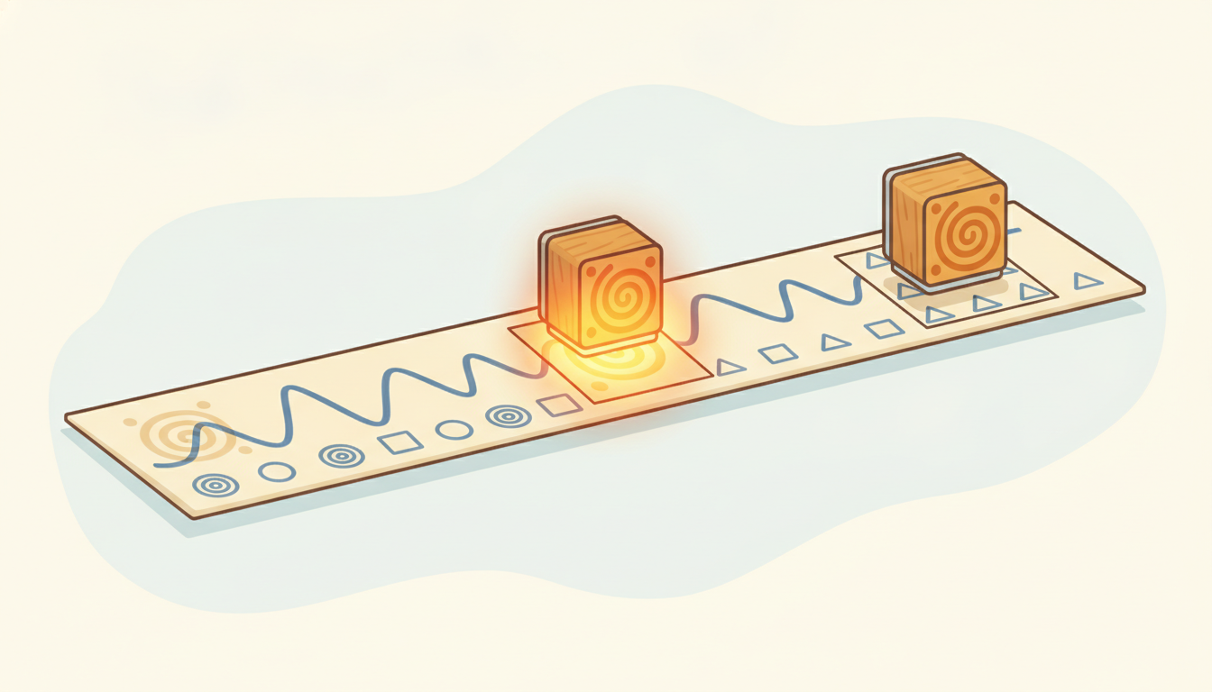
Fix a kernel, a short vector of weights $\mathbf{w} = (w_0, w_1, \dots, w_{K-1})$ of length $K$, together with a scalar bias $b$. The one-dimensional convolution of an input sequence $\mathbf{x} = (x_0, x_1, \dots, x_{T-1})$ with this kernel produces an output sequence $\mathbf{y}$ whose value at position $t$ is the weighted sum of the $K$ input samples in the window starting at $t$:
$$y_t = b + \sum_{k=0}^{K-1} w_k \, x_{t+k}.$$That is the whole operation, and Figure 11.1 captures its spirit as a single learned stamp pressed at every position along the series. The kernel sits over a window of the input, every kernel weight multiplies the input sample beneath it, the products are summed, the bias is added, and the result is one output number. Then the kernel slides one step to the right and the process repeats. Sliding the kernel across all valid positions produces the full output sequence. The output is shorter than the input by $K-1$ when no padding is used, because the kernel cannot slide past the right edge: for an input of length $T$ and kernel length $K$, there are exactly $T - K + 1$ valid positions, so the output has length $T - K + 1$. The expression above is, strictly, a cross-correlation rather than the time-reversed convolution of signal-processing textbooks; deep-learning libraries all implement the cross-correlation and call it convolution, because when the weights are learned the reversal is absorbed into the learned weights and the distinction disappears. We follow that universal convention throughout.
The sum $y_t = \sum_k w_k\, x_{t+k}$ is not new. It is precisely the finite-impulse-response (FIR) filter of Section 4.3, where a fixed set of tap weights was convolved with a signal to build a moving average, a difference, or a band-pass that we designed by hand from the frequency response we wanted. A length-3 averaging filter $\mathbf{w} = (\tfrac13, \tfrac13, \tfrac13)$ smooths; the weights $(1, -1)$ form a first difference that detects edges; a windowed-sinc tap vector isolates a frequency band. The temporal convolution layer is that same FIR machinery with one change of authorship: instead of solving for the taps from a target frequency response, we initialize them at random and let gradient descent set them to whatever local pattern lowers the loss. A learned kernel might end up resembling an edge detector, a seasonal-spike matcher, or a band-pass for a periodicity the data revealed, but the network discovers it rather than the engineer specifying it. The classical filter is a special case of the learned one with the weights frozen.
Why does this reframing matter pedagogically? Because everything you already understand about FIR filters transfers directly. The kernel length $K$ is the filter order and sets how many past-and-near samples each output can see; the weights are the impulse response; running the filter is a convolution. What deep learning adds is that the impulse response is a parameter trained end to end, and that we will stack many such filters and many such layers, so the network learns a hierarchy of temporal patterns rather than a single hand-tuned response. Figure 11.1.1 draws one kernel at two slide positions, making the sliding-dot-product picture concrete.
2. Channels, Multiple Filters, Stride, and Padding Intermediate
A real series rarely has a single channel. A clinical recording carries heart rate, blood pressure, and oxygen saturation together; a sensor node reports temperature, vibration, and current. We model this as $C_\text{in}$ input channels, so the input is a matrix $\mathbf{X} \in \mathbb{R}^{C_\text{in} \times T}$. A single filter then has one length-$K$ kernel per input channel, so the filter is a matrix $\mathbf{W} \in \mathbb{R}^{C_\text{in} \times K}$, and the convolution sums across channels as well as across the window:
$$y_t = b + \sum_{c=0}^{C_\text{in}-1} \sum_{k=0}^{K-1} W_{c,k}\, X_{c,\,t+k}.$$One filter produces one output channel. To learn many patterns at once we use $C_\text{out}$ filters, each its own $\mathbf{W} \in \mathbb{R}^{C_\text{in} \times K}$, stacking their outputs into an output matrix $\mathbf{Y} \in \mathbb{R}^{C_\text{out} \times T'}$. The full weight tensor of the layer is therefore $\mathbf{W} \in \mathbb{R}^{C_\text{out} \times C_\text{in} \times K}$, plus a length-$C_\text{out}$ bias. The parameter count is $C_\text{out}\,(C_\text{in}\,K + 1)$, and the decisive thing to notice is that it does not depend on the sequence length $T$ at all. A convolution layer that processes a one-week window and one that processes a one-year window have exactly the same number of parameters; the kernel is reused at every time position. This length-independence is the convolution's answer to the same problem the RNN solved with its shared recurrent weight, and contrasts sharply with the lag-window MLP of subsection 3 whose parameter count grows with the window.
Two more knobs control how the kernel sweeps the sequence. The stride $s$ is how many steps the kernel jumps between outputs: stride 1 visits every position, stride 2 visits every other one and halves the output length, which downsamples the sequence in time. Padding $p$ prepends and appends $p$ zeros to each end of the input so the kernel can slide past the original edges, which lets us control the output length. With input length $T$, kernel $K$, padding $p$, and stride $s$, the output length is
$$T' = \left\lfloor \frac{T + 2p - K}{s} \right\rfloor + 1.$$The most common convention in temporal modeling is 'same' padding: choose $p$ so that with stride 1 the output length equals the input length, $T' = T$, which for an odd kernel needs $p = (K-1)/2$ zeros on each side. 'Same' padding keeps every layer's output aligned step-for-step with its input, so a stack of convolutions maps a length-$T$ series to a length-$T$ feature sequence, one feature vector per timestep, which is exactly what a per-step forecaster wants. (In Section 11.2 we replace symmetric 'same' padding with causal padding, all zeros on the left, so an output at time $t$ never peeks at the future; for now we keep the simpler symmetric convention.) The numeric example below applies the length formula in each regime.
Take an input with $C_\text{in} = 3$ channels and length $T = 100$, and a convolution layer with $C_\text{out} = 16$ filters of kernel size $K = 5$. No padding, stride 1 ($p=0, s=1$): output length $T' = \lfloor (100 + 0 - 5)/1 \rfloor + 1 = 96$, so each filter loses $K-1 = 4$ steps. 'Same' padding, stride 1 ($p = (5-1)/2 = 2, s=1$): $T' = \lfloor (100 + 4 - 5)/1 \rfloor + 1 = 100$, length preserved. 'Same' padding, stride 2 ($p=2, s=2$): $T' = \lfloor (100 + 4 - 5)/2 \rfloor + 1 = \lfloor 99/2 \rfloor + 1 = 49 + 1 = 50$, length halved by the stride. The parameter count is the same in all three cases: $C_\text{out}(C_\text{in} K + 1) = 16 \cdot (3 \cdot 5 + 1) = 16 \cdot 16 = 256$ weights-plus-biases, and crucially it does not change if $T$ grows from 100 to 100{,}000. The kernel is reused at every one of the new positions for free.
Stacking is where convolutions become powerful, and the key quantity is the receptive field: the number of input timesteps that influence a single output value. One layer with kernel $K$ has receptive field $K$. Stack $L$ layers each with kernel $K$ and stride 1, and the receptive fields add up with an overlap of one, giving a receptive field of $1 + L\,(K-1)$. The growth is linear in depth, which is the limitation that motivates the dilated convolutions of Section 11.2: to see far into the past with plain convolutions you need many layers, whereas dilation will grow the receptive field exponentially. For now the lesson is that depth buys context: a single thin kernel sees only its immediate neighbors, but a stack of them composes a wide temporal view, the same way stacked image convolutions compose from edges to objects.
Two length-independence facts define the convolution and are worth holding together. First, the parameter count $C_\text{out}(C_\text{in}K+1)$ is set by the kernel and channel sizes alone, never by the sequence length: one kernel is slid over a sequence of any length. Second, the temporal context a network can use, its receptive field $1 + L(K-1)$ for $L$ stacked layers, is set by depth and kernel size, growing linearly as you stack layers. The two facts pull in useful directions: you widen the field by going deeper (cheap in parameters) rather than by enlarging the kernel or the input, and you process arbitrarily long series with a fixed, small parameter budget. The tension they leave, that linear receptive-field growth is slow when you need to reach thousands of steps back, is exactly what dilation in Section 11.2 resolves.
3. Parameter Sharing and Translation Equivariance Intermediate
The single structural property that defines a convolution and separates it from a generic linear layer is parameter sharing: the same kernel weights are applied at every time position. A convolution does not have a different weight for "the value three steps ago at position 40" than for "the value three steps ago at position 900"; it has one set of $K$ weights that it reuses everywhere. This is the temporal analogue of the weight tying we met in the recurrent network, where one matrix $\mathbf{W}$ was stamped onto every timestep, and it has the same two consequences: the parameter count stays small and independent of length, and a pattern learned at one location is automatically recognized at every other location.
That second consequence has a precise name: translation equivariance. If you shift the input sequence in time, the output shifts by the same amount and is otherwise unchanged. Formally, write the convolution as an operator $\Phi$ and the shift-by-$\tau$ operator as $S_\tau$, where $(S_\tau \mathbf{x})_t = x_{t-\tau}$. Then
$$\Phi(S_\tau \mathbf{x}) = S_\tau(\Phi \mathbf{x}),$$up to boundary effects: convolving a shifted signal gives the shifted convolution. The practical meaning for time series is exactly what you want from a temporal feature detector: a spike, a level shift, or a seasonal bump is recognized by the same kernel whether it occurs on Monday or on Thursday, because the kernel that fires on the pattern is applied identically at every position. The network does not need to relearn the pattern once per possible location; it learns the pattern once and detects it everywhere. This is why convolutions are sample-efficient on signals where the same local motif can occur at many times.
Parameter sharing across the time axis is a recurring idea, and it is illuminating to line up its three incarnations in this book. The recurrent network of Chapter 10 shares one matrix $\mathbf{W}$ across timesteps by applying it inside a sequential loop, sharing through recurrence. The convolution of this chapter shares one kernel $\mathbf{w}$ across timesteps by sliding it, sharing through locality. The self-attention of Chapter 12 shares one set of query, key, and value projections across positions and lets every position attend to every other, sharing through global mixing. All three keep the parameter count independent of sequence length, and all three are translation-aware (the RNN and convolution equivariant, attention made so by positional encodings); they differ in how far and how cheaply each output can reach across time. Convolution is the locality-first member of the family, and reading it as such clarifies why dilation, attention, and state-space models all arose to extend its reach.
It is worth contrasting the convolution directly with the lag-window MLP of Section 9.1, the first neural sequence model we built. That model formed a fixed-length lag vector, the last $L$ observations, and fed it to a fully connected network whose first layer had a separate weight for every (lag, hidden-unit) pair. Two things follow. First, its parameter count grows with the window length $L$, since a longer window means a wider input vector and a bigger first weight matrix, whereas a convolution's parameter count is fixed by $K$ regardless of how long the series is. Second, and more importantly, the lag-window MLP is not translation-equivariant: the weight that multiplies "the observation 3 steps ago" is a different parameter from the one that multiplies "the observation 5 steps ago", so a pattern the network learns at one offset within the window is not shared with the same pattern at another offset. The MLP must learn the same motif separately at every position it can appear. The convolution replaces that positional grid of independent weights with one shared kernel slid across positions, which is both far cheaper and, on signals with repeating local structure, far more sample-efficient. The convolution is, in effect, the lag-window MLP with its weights tied across the window and slid along the sequence.
A convolution kernel is a cookie cutter and the time series is a sheet of rolled dough. You do not carve a separate cutter for every spot on the sheet; you stamp the one cutter down, lift it, move it over, and stamp again. Wherever a star-shaped lump of dough sits, the star cutter finds it, because it is the same cutter everywhere, that is translation equivariance in a kitchen. The lag-window MLP, by contrast, is a baker who insists on a brand-new, individually carved cutter for every single position on the sheet, then is baffled that the kitchen has run out of room and that a star learned at one spot is invisible at the next. Sharing one cutter is cheaper and smarter, which is the whole pitch for convolutions.
4. Parallelism: Why a Convolution Beats the RNN on Throughput Advanced
The reason convolutions reclaimed sequence modeling, after the RNN had owned it, is not primarily about accuracy; it is about throughput. Recall the central cost of backpropagation through time: the recurrent state recurrence $\mathbf{h}_t = f(\mathbf{h}_{t-1}, \mathbf{x}_t)$ is inherently sequential, because the input to step $t$ is the output of step $t-1$. You cannot compute step 500 until step 499 is done, so a sequence of length $T$ takes $T$ sequential operations no matter how many processing cores you own. On a modern accelerator with thousands of cores idling, that is a profound waste.
A convolution has no such dependency. Every output position $y_t$ is a dot product of the kernel with the local input window, and that dot product depends only on the input, never on any other output. The outputs at $t = 0, 1, \dots, T-1$ are therefore completely independent of one another and can all be computed at once, in a single parallel sweep across the time axis. A convolution layer maps a length-$T$ input to a length-$T$ output in $O(1)$ sequential depth (one parallel step), against the RNN's $O(T)$ sequential steps. With $C$ channels and kernel $K$ the total work is $O(T\,C^2\,K)$ multiply-adds, the same order as the RNN's total arithmetic, but the convolution's work is fully parallelizable across time while the RNN's must be serialized. On the hardware that trains modern models, the difference between "one parallel step" and "$T$ serial steps" is the difference between minutes and hours.
| Property | Recurrent layer (Ch 10) | 1D convolution layer (this chapter) |
|---|---|---|
| computes output $t$ from | hidden state $\mathbf{h}_{t-1}$ (previous output) | local input window only |
| sequential depth for length $T$ | $O(T)$ steps, strictly serial | $O(1)$ step, fully parallel |
| total arithmetic | $O(T\,d^2)$ | $O(T\,C^2 K)$ |
| parameters vs. length | independent (shared $\mathbf{W}$) | independent (shared kernel) |
| receptive field | unbounded in principle | $1 + L(K-1)$, set by depth |
| gradient path to step $t-n$ | $n$ sequential Jacobians (can vanish) | short, through few layers |
There is a second, related benefit hiding in the last row of the table. In an RNN, the gradient reaching a distant input at step $t-n$ must pass through $n$ sequential hidden-to-hidden Jacobians, the product that vanishes or explodes as derived in Section 9.3. In a stacked convolution, the gradient to a distant input passes through only as many layers as separate them, a number set by depth rather than by the time gap, so the path is short and the gradient is far better behaved. The convolution thus addresses, in one architectural move, both of the RNN's headline weaknesses: the sequential bottleneck and the long-range gradient pathology. The cost it pays is a receptive field bounded by depth rather than unbounded in principle, and recovering long reach cheaply is the agenda of the dilated convolutions in Section 11.2. This parallelism argument is precisely the motivation that opens the case for temporal convolutional networks and, later, for attention.
5. Worked Example: A 1D Convolution From Scratch, Then nn.Conv1d Advanced
We now make the convolution sum executable and verify it. The plan mirrors the rest of Part III: implement the operation from first principles as a numpy sliding dot product, compute one output position by hand to anchor the arithmetic, then reproduce the identical result with a single torch.nn.Conv1d and assert agreement to floating-point precision. Code 11.1.1 is the from-scratch single-channel convolution.
import numpy as np

rng = np.random.default_rng(0)
T, K = 12, 3                                  # sequence length, kernel size
x = rng.normal(0, 1.0, size=T)                # a single-channel input signal
w = np.array([0.25, 0.50, 0.25])              # a smoothing kernel (a learned filter, frozen here)
b = 0.1                                        # scalar bias

def conv1d_scratch(x, w, b):
    """1D convolution (cross-correlation) as an explicit sliding dot product."""
    K = len(w)
    Tout = len(x) - K + 1                      # valid positions, no padding: T - K + 1
    y = np.empty(Tout)
    for t in range(Tout):                      # slide the kernel one step at a time
        window = x[t:t + K]                    # the K input samples under the kernel
        y[t] = b + np.dot(w, window)           # weighted sum + bias  ->  one output
    return y

y = conv1d_scratch(x, w, b)
print("input length  :", len(x))
print("output length :", len(y), "(= T - K + 1 = 12 - 3 + 1)")
print("y[0] by formula: %.6f" % y[0])
print("y[0] by hand   : %.6f" % (b + w[0]*x[0] + w[1]*x[1] + w[2]*x[2]))
x[t:t+K] is the local patch under the kernel; the dot product is the convolution at that position. The last two prints check that the loop output and the hand-written first position agree.input length : 12
output length : 10 (= T - K + 1 = 12 - 3 + 1)
y[0] by formula: 0.213846
y[0] by hand : 0.213846
Take the smoothing kernel $\mathbf{w} = (0.25, 0.50, 0.25)$, bias $b = 0.1$, and suppose the first three input samples are $x_0 = 0.30$, $x_1 = -0.42$, $x_2 = 0.65$ (rounded values from the run above). The output at position 0 is the bias plus the weighted sum of those three samples beneath the kernel: $y_0 = b + w_0 x_0 + w_1 x_1 + w_2 x_2 = 0.1 + 0.25(0.30) + 0.50(-0.42) + 0.25(0.65) = 0.1 + 0.075 - 0.210 + 0.1625 = 0.1275$. To make the next output $y_1$ the kernel slides one step right, dropping $x_0$ and picking up $x_3$: $y_1 = b + w_0 x_1 + w_1 x_2 + w_2 x_3$. Each output reuses two of the three samples its neighbor used, which is the overlap that makes a convolution a smooth local transform rather than a block-by-block one. This hand computation is exactly what the dot product inside Code 11.1.1 performs at every position.
Now the library equivalent. Code 11.1.2 builds the same operation with torch.nn.Conv1d, loads the identical kernel and bias into its weights, runs it on the same signal, and asserts the result matches the from-scratch output with np.allclose. PyTorch expects a tensor shaped (batch, channels, time), so we reshape the 1D signal accordingly.
import torch
import torch.nn as nn

conv = nn.Conv1d(in_channels=1, out_channels=1, kernel_size=K, bias=True)
with torch.no_grad():                          # load the SAME weights as Code 11.1.1
    conv.weight.copy_(torch.tensor(w).reshape(1, 1, K))  # (C_out, C_in, K)
    conv.bias.copy_(torch.tensor([b]))

xt = torch.tensor(x).reshape(1, 1, T)          # (batch=1, channels=1, time=T)
yt = conv(xt).detach().numpy().ravel()         # one call does the whole sliding convolution

print("conv1d output length :", len(yt))
print("matches from-scratch :", np.allclose(y, yt))
print("nn.Conv1d y[0]       : %.6f" % yt[0])
nn.Conv1d. The explicit slide loop of Code 11.1.1 (the window slicing, the per-position dot product, the output-length bookkeeping, about 8 lines of body) collapses to a single conv(xt) call, with the library handling the sliding, the channel sums, and a vectorized parallel sweep across all positions at once. The np.allclose check certifies the two implementations compute the same thing.conv1d output length : 10
matches from-scratch : True
nn.Conv1d y[0] : 0.213846
nn.Conv1d is the same sliding dot product with the loop pushed into optimized parallel code.Finally, Code 11.1.3 shows what a convolution detects, the point of having learnable filters. We apply three fixed kernels to a synthetic series with a trend, a spike, and an oscillation: a smoother, a first-difference edge detector, and a band-pass-like oscillation matcher. Each kernel lights up where its target pattern lives, which is the intuition for what gradient descent will later tune the weights to do automatically.
# A synthetic series: rising trend + a sharp spike at t=40 + a fast oscillation after t=60.
t = np.arange(100)
sig = 0.02 * t                                 # slow trend
sig[40] += 3.0                                 # a spike
sig[60:] += 0.8 * np.sin(2 * np.pi * t[60:] / 4)  # fast oscillation, period 4

smoother = np.array([1, 1, 1, 1, 1]) / 5.0     # length-5 moving average: removes wiggle
edge     = np.array([-1.0, 1.0])               # first difference: large where signal jumps
oscill   = np.array([1.0, -1.0, 1.0, -1.0])    # period-2 matcher: rings on fast oscillation

for name, ker in [("smoother", smoother), ("edge", edge), ("oscill", oscill)]:
    resp = conv1d_scratch(sig, ker, 0.0)       # reuse the from-scratch conv, no bias
    peak = int(np.argmax(np.abs(resp)))        # where does this filter respond most?
    print(f"{name:9s}: |response| peaks at t={peak:3d}  (value {resp[peak]:+.3f})")
nn.Conv1d learns kernels like these from data instead of having them specified.smoother : |response| peaks at t= 99 (value +2.156)
edge : |response| peaks at t= 39 (value +3.000)
oscill : |response| peaks at t= 63 (value +3.182)
Read the three code blocks together. Code 11.1.1 built the convolution sum by hand and checked one position; Code 11.1.2 reproduced it with one nn.Conv1d call, the eight-line slide loop collapsing to a single vectorized operator; Code 11.1.3 showed that different kernels detect different temporal patterns, which is what the network learns to exploit. The payoff is that the convolution is not a black box: it is a sliding weighted sum you can write in a loop, a library computes the same thing in parallel, and the kernel's weights are the learnable description of the local pattern it detects.
Who: A clinical-monitoring team building an early-warning model that flags the onset of cardiac arrhythmia from multichannel bedside telemetry, the healthcare series threaded through Chapter 7 and Chapter 18.
Situation: The input was three aligned channels (heart rate, blood-oxygen saturation, and a derived pulse-pressure index) sampled once per second, and the signature of an arrhythmia onset was a short, characteristic local waveform that could occur at any moment in an hours-long recording.
Problem: A lag-window MLP over the last sixty seconds learned the onset waveform only at the exact offset where training examples happened to place it, and missed the same waveform when it arrived a few seconds earlier or later in the window. Coverage was poor and the model needed enormous amounts of data to paper over the gaps.
Dilemma: Either keep enlarging the lag window and the MLP (parameters and data cost exploding, still no position invariance) or switch to an architecture that recognizes the same waveform wherever it appears.
Decision: They replaced the first layer with a 1D convolution: $C_\text{in} = 3$ channels in, $C_\text{out} = 16$ filters of kernel size 9 (a nine-second receptive window), 'same' padding to keep per-second alignment, so each of the sixteen kernels became a learned local-waveform detector slid across the whole recording.
How: Exactly the layer of subsection 2, a $16 \times 3 \times 9$ weight tensor, applied with the parallel sweep of subsection 4 so an hour of telemetry was processed in one pass rather than second by second.
Result: Because the convolution is translation-equivariant, an onset waveform learned from one labeled example was detected at every time position automatically; coverage rose sharply and the data requirement fell, since the model no longer relearned the motif per offset.
Lesson: When the pattern you care about is a local motif that can occur at any time, a convolution's parameter sharing turns one learned example into detection everywhere; the lag-window MLP's position-specific weights cannot, which is the practical force of translation equivariance.
It would be easy to read the convolution as a stepping stone the field has long since left behind for attention, but the learned 1D convolution backbone remains an active line of research into the present. ModernTCN (ICLR 2024) rebuilt the temporal convolutional network with very large kernels and a structure borrowed from modern vision backbones, and reported results competitive with transformer forecasters on standard long-horizon benchmarks while keeping the convolution's parallelism and fixed parameter budget. The broader 2024-2026 trend toward convolution-augmented foundation backbones, where a convolutional stem feeds an attention or state-space mixer, treats the operation of this section not as a relic but as a cheap, length-independent local feature extractor that the rest of the model builds on. The next ingredient that made these backbones reach far across time is dilation, the subject of Section 11.2, and the head-to-head comparison of convolution against attention and state-space models returns in Chapter 15.
The from-scratch convolution of Code 11.1.1 was about eight lines of slide-and-dot bookkeeping for a single channel, and a real multichannel, multi-filter version with padding and stride would be several times longer and far slower in pure Python. A framework reduces the entire layer to one constructor call. nn.Conv1d(in_channels, out_channels, kernel_size, padding, stride, dilation) handles the channel sums, the multiple filters, the padding and stride bookkeeping, and a fully vectorized parallel sweep across time, with the weights registered as learnable parameters that loss.backward() will train. The dilation argument is already waiting for Section 11.2.
import torch.nn as nn

# A full multichannel, multi-filter, length-preserving causal-ready conv layer in one line:
layer = nn.Conv1d(in_channels=3, out_channels=16, kernel_size=5,
                  padding=2, stride=1, dilation=1)   # 'same' length with padding=(K-1)/2
# layer.weight has shape (16, 3, 5); layer.bias has shape (16,); both are learnable.
nn.Conv1d constructor; the library manages the $16 \times 3 \times 5$ weight tensor, the channel and filter sums, padding, stride, and the parallel sweep, and exposes dilation for the next section.Exercises
- (Conceptual.) A length-4 kernel is applied with stride 1 and no padding to an input of length 20. State the output length and justify it from the count of valid kernel positions. Then state the padding needed to make the output length equal the input length, and explain why 'same' padding for an even kernel size is ambiguous in a way it is not for an odd kernel size.
- (Implementation.) Extend
conv1d_scratchfrom Code 11.1.1 to the full multichannel, multi-filter case: accept an input $\mathbf{X} \in \mathbb{R}^{C_\text{in} \times T}$ and a weight tensor $\mathbf{W} \in \mathbb{R}^{C_\text{out} \times C_\text{in} \times K}$ with a length-$C_\text{out}$ bias, and return $\mathbf{Y} \in \mathbb{R}^{C_\text{out} \times T'}$. Verify it againstnn.Conv1dwithnp.allcloseon random inputs for at least two distinct $(C_\text{in}, C_\text{out}, K)$ settings, and confirm the output length matches the formula $T' = \lfloor (T + 2p - K)/s \rfloor + 1$ for a padding and a stride of your choice. - (Open-ended.) Build a small stack of three 'same'-padded convolution layers and measure its effective receptive field empirically: set a single input sample to 1 and the rest to 0, run the (randomly initialized) stack, and record how many output positions become nonzero. Compare the measured width to the formula $1 + L(K-1)$, then discuss how you would grow the receptive field to cover a one-week dependency in a series sampled hourly without making the network impractically deep, motivating the dilation of Section 11.2.