Open Challenges and Research Frontiers

"I have spent thirty-six chapters insisting that the future can be modeled, and now, with the margin running out, I will confess the obvious: every answer I gave opened two questions, and the two questions opened four. The arrow of time, it turns out, points at the reader. Go on. The interesting part starts where the pages stop."

A Book About Time, Finally Running Out of Pages but Not of Questions

In Section 36.4 we priced the road to general temporal intelligence through scaling laws and the accuracy-versus-cost frontier. That was the forward-looking picture. This section closes the loop by looking both ways at once: back across the entire book to name the single thread that ties it together, and forward across the research horizon to name what is still unsolved. Every symbol we use here was defined earlier and is collected in Appendix A; we will not introduce new machinery, only assemble what you already hold. Consider this less a section than a coda.

1. The Synthesis: One Problem, One Toolkit, One Thread

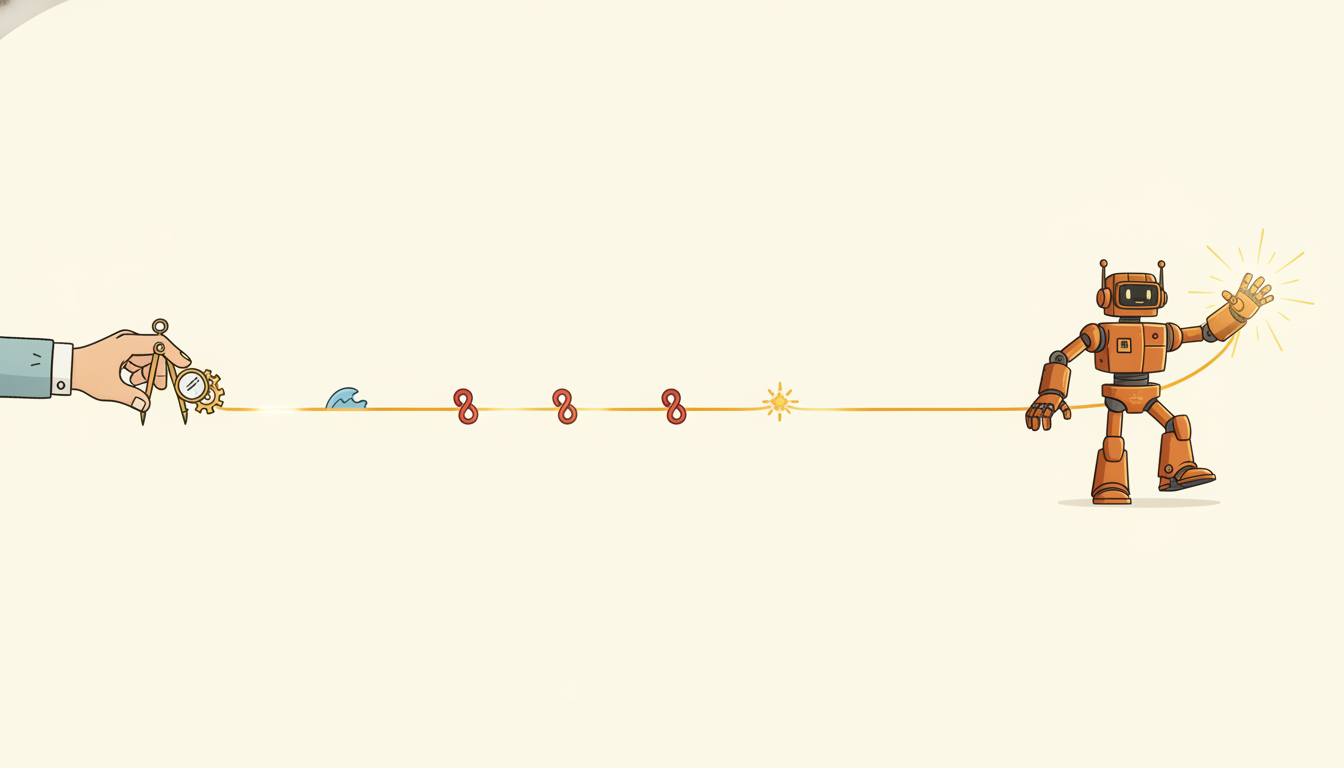
Here is the thesis the book has been building toward, stated plainly now that the evidence is in. Prediction, reasoning, and decision making over time are one problem. Forecasting asks what comes next; reasoning asks what an observed sequence implies about hidden structure; decision making asks which action to take so that the future is better than it would otherwise be. These look like different fields with different conferences, but they share a single skeleton: a latent state that summarizes the relevant past, an update rule that carries that state forward as new observations arrive, and a readout that turns the state into whatever the task needs, a prediction, an inference, or an action. Change the readout and the loss and you change the task; the loop underneath is the same loop. That is why one toolkit, the recurrence, the latent variable, the differentiable loss, the policy, and the calibrated uncertainty around all of them, serves the entire span from ARIMA to autonomous agents.

The clearest proof of the thesis is the single arc the book has called the temporal thread: one idea, recursive state estimation, reappearing at every level of the curriculum, each time more learned and more capable than the last, never abandoning the structure that made the first version work. Follow it from start to finish.

• The Kalman filter (Section 7.6): a hand-specified linear-Gaussian recurrence $\mathbf{x}_t = \mathbf{A}\mathbf{x}_{t-1} + \mathbf{w}_t$, $\mathbf{z}_t = \mathbf{H}\mathbf{x}_t + \mathbf{v}_t$, with an optimal closed-form update for the belief over the hidden state. The model is given; only the state is inferred.
• The recurrent network (Section 10.5): the same loop $\mathbf{h}_t = f(\mathbf{h}_{t-1}, \mathbf{x}_t)$, but now $f$ is learned by gradient descent rather than derived from physics. The Kalman filter's hand-built transition becomes a trained nonlinearity; the optimal-update calculus becomes backpropagation through time.
• The structured state-space model (Section 13.6): the recurrence made linear again, on purpose, so it can be run as a parallel scan, recovering the Kalman filter's analytic tractability while keeping the RNN's learned parameters. S4 and Mamba are Kalman filters that learned their own dynamics and can be trained at the scale of a Transformer.
• The belief-state agent (Section 23.4): the same recursive state now carries a belief over a hidden world, and the readout is no longer a prediction but the input to a decision. The filter's posterior becomes the agent's memory.
• The sequence-model policy (Section 28.5): decision making itself reframed as sequence modeling. The Decision Transformer treats a trajectory of returns, states, and actions as a sequence to be completed, so the policy is a forecaster and the forecaster is a policy. The thread has closed a circle: prediction and decision are literally the same model.
• The foundation temporal agent (Section 36.3): one large pretrained model that perceives, remembers, predicts, and acts across domains, carrying the recurrence, the belief, and the policy inside a single set of weights. The hand-built filter of Chapter 7 has become a general agent, and it is still, at heart, a state that summarizes the past and a rule that carries it forward.

Read that list top to bottom and you have read the book's argument in one breath. Nothing was thrown away as the thread advanced; each stage kept the previous stage's structure and only relaxed an assumption, the model becomes learned, the dynamics become nonlinear then re-linearized for scale, the readout becomes an action, the training becomes self-supervised pretraining. The figure below draws the thread as the single spine it is.

2. The Open Challenges, Honestly

A finale that only celebrated would be dishonest. The thread is real and the toolkit is powerful, and it is also true that every major capability in this book degrades in ways the field has not solved. Naming those failures precisely is the most useful thing a closing section can do, because unsolved problems are where the reader's own contribution will come from. Here are the seven that matter most, each tied to where in the book you met the capability it limits.

• Genuine long-range reasoning and credit assignment. Backpropagation through time (Section 9.3) assigns credit across a sequence, but the Jacobian product that carries gradient across thousands of steps still vanishes or explodes, and attention's quadratic cost caps the context in practice. Models that appear to reason over long horizons often pattern-match on recent context. Reliable credit assignment over truly long temporal gaps, the kind a person uses to connect a cause to an effect months later, remains open.
• Robustness to non-stationarity and distribution shift. This is the field's perennial hard problem, the one assumption that almost every method quietly relies on and the real world almost never grants. Stationarity was defined in Chapter 3, violated and tested throughout Part II, and confronted head-on as concept drift in Chapter 20. We have detectors, adaptation rules, and online updates, and we still do not have a model that gracefully handles a regime it has never seen. A forecaster trained on one decade and deployed in the next is, in general, on its own.
• Calibrated, decision-aware uncertainty. Chapter 19 gave us conformal prediction and probabilistic heads that produce honest intervals under exchangeability, but exchangeability is exactly what non-stationarity breaks, and a calibrated interval is not the same as a useful one. An interval that is correct on average can still be uninformative for the one decision that matters. Connecting uncertainty to the downstream decision, so that the model is uncertain about the things the decision is sensitive to, is largely unsolved.
• Causality from observational temporal data. Granger causality (Chapter 6) and the temporal-reasoning machinery of Chapter 30 detect predictive structure, but predictive structure is not causal structure, and an agent that acts on a spurious correlation will be punished by the very intervention it performs. Recovering genuine cause from passively observed time series, without the luxury of randomized experiments, is one of the deepest open problems and the one most relevant to agents that act.
• Data scarcity for temporal foundation models. The foundation models of Chapter 15 need scale, but time-series data is fragmented, proprietary, irregularly sampled, and far less abundant than text or images. There is no temporal equivalent of the open web. Pretraining a general temporal model is gated as much by data as by compute.
• Evaluation that cannot be gamed. Leakage (Chapter 2) is the original sin of temporal evaluation, and it has only become subtler as models grow. Benchmarks saturate, get memorized, and reward the wrong thing; a model can top a leaderboard and fail in deployment because the leaderboard measured the past, not the future. Designing temporal benchmarks that resist gaming and actually predict deployment performance is an unglamorous, essential, open problem.
• Safety and alignment of agents that act over time. An agent that acts changes the distribution of the data it later sees (Chapter 25), so its mistakes compound rather than average out, and the trustworthiness machinery of Chapter 33 was largely built for models that predict, not models that intervene. Specifying what a temporal agent should optimize, bounding what it can do while it learns, and keeping it aligned as it reshapes its own future are open in both theory and practice.

3. The Frontiers: 2025, 2026, and Beyond

The open challenges define the destination; the frontiers are where the field is actually pushing right now. Four lines of work are the most active as this edition goes to press, each one a direct assault on the challenges above.

Continual and lifelong agents. The online and continual learning of Chapter 20 is being pushed toward agents that learn for their entire deployment without catastrophic forgetting, accumulating skills the way a person accumulates experience. Test-time training, streaming adaptation, and memory-augmented agents that write durable experience to an external store are the concrete instances, and they target non-stationarity and data scarcity at once.

World models for planning. The Dreamer line (Dreamer V3, Hafner et al.) and MuZero's learned-model planning, introduced in Chapter 29, are scaling into general world models that an agent can roll forward to plan, and 2024 to 2026 has seen video-prediction world models and large interactive simulators turned into planning substrates. A model that can imagine the consequences of its actions is the most direct path to safe, sample-efficient decision making.

Neuro-symbolic temporal reasoning. The reasoning machinery of Chapter 30 is being fused with the pattern strength of large sequence models, so that a system can both learn from data and respect explicit temporal logic and causal constraints. This is the most promising attack on the long-range-reasoning and causality challenges together: let the network see the pattern and let the symbols keep it honest.

Temporal AI for science and climate. Perhaps the frontier with the highest stakes. Foundation-scale temporal models are now central to weather and climate forecasting (GraphCast, GenCast, and the wave of AI weather models that match or beat numerical solvers at a fraction of the cost), to epidemiology, and to the physical and life sciences, where the data is a time series and the decision is consequential. This is where the book's whole argument, that a forecast exists to inform a decision, meets problems that genuinely matter.

4. The Enduring Principles to Carry

Architectures will turn over; the Transformer was not the last word and neither will be whatever follows the state-space wave. What does not turn over is a short list of principles that were true for ARIMA and remain true for foundation agents. Carry these out of the book and you will be right far more often than the architecture of the month suggests.

5. The Closing Capstone: A Forecast Tied to a Decision

The whole book in one idea is this: a forecast exists to inform a decision, and the two together, under honest uncertainty, are the unit of temporal intelligence. The running datasets that threaded the book, the finance returns series of Part II, the irregularly-sampled healthcare vitals of Part II and Part III, and the sensor/IoT telemetry of Part II and Part VII, were chosen so that you could carry one problem all the way from a classical model to a deployed agent. The capstone project asks you to do exactly that: take one of those series, build a forecaster, attach an uncertainty estimate, and turn the pair into a decision, then evaluate the decision, not just the forecast.

To make the unit concrete, here is the book in miniature: a forecast with an uncertainty band, and a decision that uses the band rather than the point. The from-scratch version makes the logic explicit, then a one-line library call shows the production path.

import numpy as np

# A forecast is not a number; it is a distribution. Here: a predicted demand
# with a calibrated 90% interval (from a conformal or quantile model, Ch 19).
point_forecast = 1000.0          # expected demand for next period
lower, upper   = 880.0, 1180.0   # calibrated 90% interval (NOT a guess)

# A decision uses the WHOLE distribution, not just the point. The classic
# newsvendor: order quantity balances the cost of too little vs too much.
cost_under = 5.0                 # cost per unit of unmet demand (stockout)
cost_over  = 1.0                 # cost per unit of leftover stock
critical_ratio = cost_under / (cost_under + cost_over)   # = 0.833...

# Decision-aware: order at the critical-ratio quantile of the predictive
# distribution, NOT at the point forecast. Approximate the quantile from the
# interval (treat the 90% band as spanning the 5th-95th percentiles).
def interval_quantile(lo, hi, q):
    """Linear-interpolate a quantile from a 5%-95% predictive interval."""
    return lo + (hi - lo) * (q - 0.05) / 0.90        # maps q in [0.05, 0.95]

order = interval_quantile(lower, upper, critical_ratio)
print(f"point forecast      : {point_forecast:.0f}")
print(f"critical ratio      : {critical_ratio:.3f}")
print(f"decision (order qty) : {order:.0f}")   # above the point, because stockouts hurt more

The point of Code 36.5.1 is the line that orders above the point forecast: the decision moved because the uncertainty and the asymmetric cost demanded it, which is the entire reason we quantify uncertainty in the first place. A point forecast plugged straight into an order would have under-ordered and eaten stockout costs. In production you would not interpolate quantiles by hand; a forecasting library gives you the predictive quantiles directly, and the newsvendor solution is a one-liner on top.

# Production path: a probabilistic forecaster yields quantiles directly,
# and the decision is one line on top of them.
from scipy.stats import norm

# A library model (e.g. a quantile/conformal forecaster from Ch 19, or a
# DeepAR/TimesFM head) returns a calibrated predictive distribution.
predictive = norm(loc=1000.0, scale=90.0)        # stand-in for the fitted forecaster

order = predictive.ppf(critical_ratio)           # newsvendor optimum = critical-ratio quantile
print(f"decision (order qty) : {order:.0f}")

Exercises

These exercises close the book the way the chapters did, with one conceptual, one implementation, and one open-ended task. Selected solutions are in Appendix G.

1. (Conceptual.) The temporal thread of Section 1 claims that the Kalman filter, the RNN, the structured state-space model, the belief-state agent, the Decision Transformer, and the foundation agent are "one loop, increasingly learned." For each adjacent pair in that list, name the single assumption that is relaxed when you move from the earlier to the later member (for example, Kalman to RNN relaxes "dynamics are given and linear-Gaussian"). Then argue in two or three sentences why nothing essential to the loop is lost at any step.
2. (Implementation.) Extend Code 36.5.1. Replace the single fixed interval with a small predictive distribution sampled from a non-stationary process (draw demand from a normal whose mean drifts upward over 50 periods), recompute the newsvendor order at each step using the critical-ratio quantile, and compare the total cost of (a) ordering at the point forecast versus (b) ordering at the decision-aware quantile. Report which wins and by how much, and connect the result to the "quantify uncertainty, decision-aware" principle of Section 4 and to the drift discussion of Chapter 20.
3. (Open-ended.) Pick one of the seven open challenges in Section 2 and write a one-page research proposal: state the problem precisely, identify which chapter's machinery you would start from, name one 2025 to 2026 method from Section 3 you would build on, and describe a single experiment, on one of the book's three running datasets, that would constitute progress. Be honest about how you would detect leakage and how you would beat the simple baseline.