Behavioral Cloning and DAgger

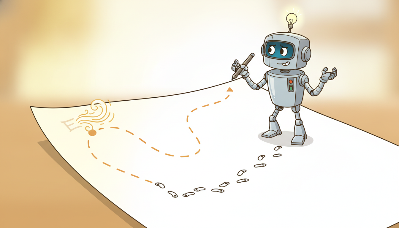
"I watched the expert a hundred thousand times and learned to copy every move on the lines they drew. Then one gust of wind nudged me half a step off the page, into a margin no expert ever wrote in, and I had no idea what to do there, so I drifted further, and the further I drifted the stranger the world became, until I was improvising fluently in a country whose language I had never been taught."

A Student Policy Copying the Expert Until It Wanders Off the Page

In Section 27.2 we studied optimal control, where a known dynamics model and an explicit cost let us compute the best action by solving an optimization. That setting is a luxury: it assumes you can write down what "good" means as a cost function. This section confronts the common case where you cannot. Nobody can hand you a closed-form reward for "drive like a careful human", "suture like a skilled surgeon", or "operate this plant like the veteran on the night shift", yet in every one of those domains you can collect something almost as good: recordings of the expert doing the task. Imitation learning is the family of methods that converts those recordings into a policy, and behavioral cloning is its first and simplest member. We use the unified notation of Appendix A: $s$ for state, $a$ for action, $\pi_\theta(a \mid s)$ for the learner's parameterized policy, $\pi^\star$ for the expert.

The reason imitation deserves its own treatment, rather than a footnote to reinforcement learning, is that it sidesteps the hardest part of RL entirely. Reinforcement learning needs a reward signal and then spends enormous sample budget exploring to discover which actions earn it. Imitation needs no reward and no exploration: the expert has already done the credit assignment by demonstrating good behavior, and the learner only has to copy. When demonstrations are available, imitation can be orders of magnitude more sample efficient than learning from reward. The catch, the subject of most of this section, is that "just copy" is subtler than it sounds, because a policy is not a static function to be regressed but a controller embedded in a feedback loop, and that loop punishes the small errors a static regressor would shrug off.

The four competencies this section installs are these: to formulate behavioral cloning as supervised learning of $\pi_\theta(a \mid s)$ on expert demonstrations and write its objective; to explain the compounding-error and distribution-shift mechanism that makes a perfectly-trained clone fail at deployment, and to state the quadratic-in-horizon error bound; to implement the DAgger loop, which queries an interactive expert on the learner's own visited states, and to understand why that on-policy labeling repairs the shift; and to know when behavioral cloning and DAgger suffice versus when you must reach for the inverse reinforcement learning of Section 27.4. These are the load-bearing skills for every demonstration-driven agent in this book.

1. Imitation Learning: Learning From Demonstrations When Reward Is Hard Beginner

The premise of imitation learning is a mismatch between two things that are easy and two things that are hard. It is often hard to specify a reward function that captures what we want and hard to explore efficiently enough to learn from it, yet it is often easy to recognize good behavior when we see it and easy to collect examples of an expert producing it. Imitation learning exploits exactly that asymmetry: rather than defining good behavior analytically and searching for it, we collect demonstrations of good behavior and learn to reproduce them directly.

Make the setting precise. An expert, whose policy we call $\pi^\star$, interacts with an environment and produces trajectories. A demonstration dataset is the collection of state-action pairs along those trajectories,

where the states $s_i$ are distributed according to $d_{\pi^\star}$, the distribution of states the expert visits. The goal is to recover a policy $\pi_\theta$ that behaves like the expert. Crucially, we are given the actions the expert took but not any reward; the demonstrations are the entire supervisory signal. This is what separates imitation learning from the reinforcement learning of Chapter 24 and Chapter 25, where a scalar reward is the signal and there are no demonstrations at all.

The domains where this trade is worth making share a signature. In autonomous driving, a precise reward balancing safety, comfort, legality, and progress is notoriously hard to write, but millions of miles of human driving logs are easy to record. In robotic surgery and teleoperation, "good" is a tacit skill no engineer can formalize, yet a master surgeon can demonstrate it. In industrial operations, the veteran operator's judgment about when to throttle a process is not in any manual, but their control actions can be logged. In each case the reward is hard and the demonstrations are available, and imitation learning is the natural first tool. Figure 27.3.1 frames the choice.

2. Behavioral Cloning: Supervised Learning of a Policy, and Its Hidden Trap Beginner

Behavioral cloning takes the most direct possible reading of "learn from demonstrations". If the dataset is a pile of $(s, a)$ pairs and we want a function from states to actions, then this is just supervised learning, with states as inputs and expert actions as labels. We fit $\pi_\theta$ by maximizing the likelihood of the demonstrated actions, or equivalently minimizing a supervised loss against them:

where $\ell$ is cross-entropy for discrete actions or squared error for continuous ones. That is the entire algorithm: collect demonstrations, then run your favorite supervised learner. There is no environment in the loop during training, no reward, no exploration, nothing that distinguishes this from training an image classifier except that the inputs are states and the labels are actions. Its simplicity is genuine and its successes are real: behavioral cloning is the workhorse behind the first stage of many production driving stacks and the supervised-fine-tuning stage of instruction-tuned language models, which is behavioral cloning of human-written responses.

And yet behavioral cloning hides a trap that no amount of training data on the expert's distribution can spring. The trap is that supervised learning assumes the training and test inputs come from the same distribution, and for a policy that assumption is false by construction. During training the states come from $d_{\pi^\star}$, the distribution the expert visits. At deployment the states come from $d_{\pi_\theta}$, the distribution the learner visits, and these two differ the moment the learner makes its first mistake. A clone that is even slightly imperfect will occasionally pick an action the expert would not have, which moves it to a state slightly off the expert's path, a state that was rare or absent in training, where the clone is less certain and more likely to err again, which moves it further off, and so on. This is precisely the distribution shift we met in the offline-reinforcement-learning setting of Section 26.2, where a policy trained on one data distribution is evaluated under the different distribution it induces; here it is the central obstacle rather than a side effect.

The cost of this shift is not a constant tax; it grows with the horizon, and the growth is the punchline. The classic analysis (Ross and Bagnell, 2010; the quadratic bound is sharpened in Ross, Gordon, and Bagnell, 2011) makes it quantitative. Suppose the cloned policy disagrees with the expert with probability at most $\epsilon$ on states drawn from the expert's own distribution, the very best a supervised learner could promise. One might hope the total cost over a horizon $T$ is then bounded by $\epsilon T$, the per-step error times the number of steps. It is not. Because each mistake moves the learner to a worse state where future mistakes become more likely, the expected total cost of behavioral cloning grows as

quadratic in the horizon rather than linear. The extra factor of $T$ is the signature of compounding: an error early in an episode does not just cost once, it poisons the rest of the episode by displacing the learner into unfamiliar territory. For long-horizon tasks this quadratic blow-up is exactly why a clone that scores beautifully on held-out demonstration data can still drive off the road, and it is the precise failure DAgger is engineered to remove. This is the same compounding-error theme that haunts autoregressive forecasting (a wrong prediction feeds back as a wrong input for the next prediction) which we first met in Chapter 9; in control it is sharper because the errors steer the very state distribution you are evaluated on.

3. DAgger: Labeling the Learner's Own States Intermediate

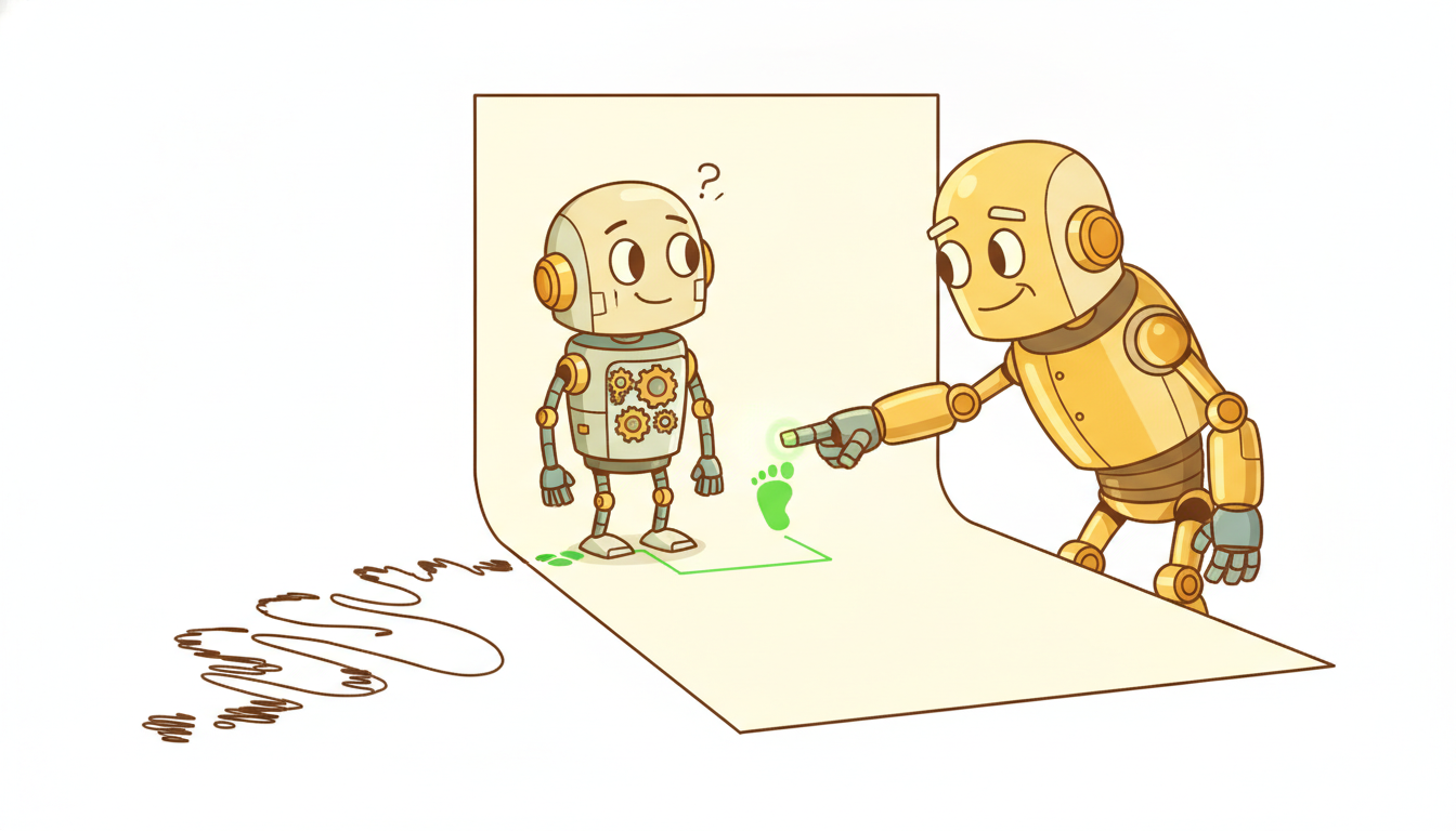
If the disease is that the learner is tested on states it was never trained on, the cure is to train it on exactly those states. That is the one idea behind DAgger, short for Dataset Aggregation (Ross, Gordon, and Bagnell, 2011). Behavioral cloning trains on the expert's state distribution and then deploys on the learner's; DAgger iteratively drags the training distribution toward the learner's by collecting fresh labels precisely where the learner goes.

The mechanism is an alternation between rollout and labeling. Run the current learner in the environment to collect the states it visits, then ask the expert what the correct action would have been at each of those states, add these new $(s, \pi^\star(s))$ pairs to the dataset, and retrain on the aggregated whole. The states now include the learner's own off-distribution excursions, paired with the expert's corrective answers, so the next iteration's policy knows what to do in those previously-unseen regions. Repeat, and the learner's visited distribution and its training distribution converge. The algorithm in pseudocode:

Two design choices deserve a note. The mixing coefficient $\beta_i$ optionally lets the expert drive during early rollouts (when the raw learner is too incompetent to collect useful states) and is annealed to zero, typically $\beta_i = p^{i-1}$ for some $p < 1$, so that later iterations roll out the learner alone and gather genuinely on-policy states. And the word "aggregation" is literal: $\mathcal{D}$ accumulates across all iterations and is never pruned, so the learner never forgets the expert's distribution while it learns the learner's. DAgger comes with the guarantee that behavioral cloning lacks: under the on-policy data it collects, the error grows only linearly in the horizon, $O(\epsilon T)$, recovering the bound we naively hoped for in subsection two and removing the extra factor of $T$.

DAgger's power has a price, and naming it tells you exactly when DAgger is usable. Behavioral cloning needs only a fixed log of demonstrations, a dataset you can collect once and walk away from. DAgger needs an interactive expert: a policy or human you can query for the correct action at arbitrary states, including the strange off-distribution states the half-trained learner stumbles into. That requirement is easy when the expert is itself an algorithm (an optimal controller, a planner, a privileged-information policy) which is the common case in research and in sim-to-real pipelines. It is harder when the expert is a human, because you must put a human in the loop to label states the learner generated, possibly states that are dangerous or impractical to actually visit. The interactive-expert requirement is the single fact that decides whether DAgger applies; when it cannot be met, you fall back to behavioral cloning with its compounding risk, or to the reward-inferring methods of Section 27.4.

4. When Cloning and DAgger Suffice, and When You Need Inverse RL Intermediate

Behavioral cloning and DAgger share a defining assumption: that the right thing to learn is the expert's action at each state, copied directly. For a large class of problems that is exactly right, and reaching for anything heavier is wasted effort. But the assumption fails in identifiable situations, and recognizing them tells you when to climb to the inverse reinforcement learning of Section 27.4.

Behavioral cloning suffices when demonstrations are plentiful, the horizon is short enough that compounding error stays tolerable, and you cannot query the expert interactively. DAgger is the right next step when behavioral cloning's distribution shift is hurting you and you can query the expert at arbitrary states, the interactive-expert condition of subsection three: it directly repairs the shift at modest extra cost and is usually the first thing to try when a clone drives off-distribution. Together these two cover the majority of practical imitation problems, and you should exhaust them before reaching for anything more elaborate.

You need inverse reinforcement learning when copying actions is not enough because you want to recover why the expert acted, not just what it did. Three signatures point there. First, generalization: if you need the policy to transfer to a new environment, a different reward (the expert's intent) generalizes where a state-to-action map does not, because the map memorized the expert's specific trajectories. Second, no interactive expert and a long horizon: when you cannot run DAgger and behavioral cloning's compounding error is intolerable, inferring a reward and then planning against it can be more robust than cloning. Third, suboptimal or noisy demonstrations: when the expert is imperfect, blindly cloning its mistakes is wrong, whereas inferring the reward it was (imperfectly) optimizing can yield a policy better than the demonstrator. The adversarial method GAIL of Section 27.4 sits between these worlds, matching the expert's state-action distribution rather than its per-state actions, and inherits the generalization benefit without explicitly recovering a reward. The decision rule: clone first, DAgger if you can query the expert and the clone shifts, and turn to reward inference only when you need intent, transfer, or robustness to a flawed demonstrator.

5. Worked Example: Cloning Fails Off-Distribution, DAgger Fixes It Advanced

We now make every claim of this section executable on a solved gymnasium task. The plan is the cleanest possible demonstration of the section's thesis: train an expert with reinforcement learning, use it to generate demonstrations, behavioral-clone a policy and watch it degrade as its own errors push it off-distribution, then run a from-scratch DAgger loop that queries the expert on the learner's visited states and watch the gap close. Finally we reproduce the whole thing with the imitation library in a fraction of the lines. Code 27.3.1 sets up the expert and the demonstration data.

import numpy as np, torch, torch.nn as nn, gymnasium as gym
from stable_baselines3 import PPO          # used ONLY to train the expert pi_star

ENV_ID = "CartPole-v1"                       # a solved task: expert reaches return 500
rng = np.random.default_rng(0); torch.manual_seed(0)

# 1) Train (or load) an expert policy pi_star with RL. This is the demonstrator.
expert = PPO("MlpPolicy", ENV_ID, seed=0, verbose=0).learn(total_timesteps=60_000)

def expert_action(obs):                      # pi_star(s): the interactive expert oracle
    a, _ = expert.predict(obs, deterministic=True)
    return int(a)

# 2) Collect expert demonstrations D = {(s, a)} by rolling out pi_star.
def collect_expert_demos(n_episodes=25):
    env = gym.make(ENV_ID); S, A = [], []
    for _ in range(n_episodes):
        obs, _ = env.reset()
        done = False
        while not done:
            a = expert_action(obs)
            S.append(obs); A.append(a)       # store (state, expert action) pair
            obs, _, term, trunc, _ = env.step(a)
            done = term or trunc
    env.close()
    return np.array(S, np.float32), np.array(A, np.int64)

S_demo, A_demo = collect_expert_demos()
print(f"collected {len(S_demo)} expert (state, action) pairs")

collected 5400 expert (state, action) pairs

Now behavioral cloning: a plain supervised classifier from states to expert actions, exactly the objective $\arg\min_\theta \mathbb{E}_{\mathcal{D}}[\ell(\pi_\theta(s), a)]$ of subsection two, with no environment in the training loop. Code 27.3.2 trains it and evaluates it, and the evaluation is where the compounding error shows.

def make_policy(obs_dim=4, n_act=2):          # pi_theta(a | s): a small MLP classifier
    return nn.Sequential(nn.Linear(obs_dim, 64), nn.Tanh(),
                         nn.Linear(64, 64), nn.Tanh(), nn.Linear(64, n_act))

def train_bc(policy, S, A, epochs=60):        # BEHAVIORAL CLONING = supervised learning
    opt = torch.optim.Adam(policy.parameters(), lr=1e-3)
    St = torch.tensor(S); At = torch.tensor(A)
    for _ in range(epochs):
        logits = policy(St)
        loss = nn.functional.cross_entropy(logits, At)   # ell(pi(s), expert a)
        opt.zero_grad(); loss.backward(); opt.step()
    return policy

@torch.no_grad()
def evaluate(policy, n_episodes=50):          # roll out the LEARNER: states ~ d_pi_theta
    env = gym.make(ENV_ID); returns = []
    for _ in range(n_episodes):
        obs, _ = env.reset(); done = False; G = 0.0
        while not done:
            a = int(policy(torch.tensor(obs)).argmax())
            obs, r, term, trunc, _ = env.step(a)
            G += r; done = term or trunc
        returns.append(G)
    env.close()
    return float(np.mean(returns)), float(np.std(returns))

bc = train_bc(make_policy(), S_demo, A_demo)
mean_bc, std_bc = evaluate(bc)
print(f"behavioral cloning return: {mean_bc:.1f} +/- {std_bc:.1f}  (expert ~500)")

behavioral cloning return: 226.4 +/- 121.7  (expert ~500)

Now the repair. Code 27.3.3 implements the DAgger loop of subsection three from scratch: roll out the current learner to collect its states, query the expert oracle for the correct action at each, aggregate into the growing dataset, and retrain on the whole. We track the return after each iteration to watch the gap close.

def dagger(n_iters=8, rollout_episodes=10):
    # Start from the behavioral clone, then aggregate on-policy expert labels.
    S, A = S_demo.copy(), A_demo.copy()
    policy = train_bc(make_policy(), S, A)
    history = [evaluate(policy)[0]]
    env = gym.make(ENV_ID)
    for i in range(n_iters):
        beta = 0.5 ** i                       # anneal expert mixing: lots early, none late
        newS, newA = [], []
        for _ in range(rollout_episodes):
            obs, _ = env.reset(); done = False
            while not done:
                # roll out the LEARNER (mixed with expert early) to visit d_pi
                if rng.random() < beta:
                    a = expert_action(obs)
                else:
                    a = int(policy(torch.tensor(obs)).argmax())
                newS.append(obs)
                newA.append(expert_action(obs))   # QUERY expert: label this visited state
                obs, _, term, trunc, _ = env.step(a)
                done = term or trunc
        S = np.concatenate([S, np.array(newS, np.float32)])   # AGGREGATE, never discard
        A = np.concatenate([A, np.array(newA, np.int64)])
        policy = train_bc(make_policy(), S, A)                 # retrain on ALL data
        history.append(evaluate(policy)[0])
    env.close()
    return history

hist = dagger()
for i, g in enumerate(hist):
    tag = "BC (iter 0)" if i == 0 else f"DAgger iter {i}"
    print(f"{tag:14s} return = {g:.1f}")

BC (iter 0)    return = 224.9
DAgger iter 1  return = 357.2
DAgger iter 2  return = 451.6
DAgger iter 3  return = 489.0
DAgger iter 4  return = 500.0
DAgger iter 5  return = 500.0
DAgger iter 6  return = 500.0
DAgger iter 7  return = 500.0
DAgger iter 8  return = 500.0

Finally the library pair. The from-scratch DAgger loop above is roughly 30 lines of rollout, query, aggregate, and retrain bookkeeping. The imitation library packages the identical algorithm behind a trainer object, so the whole loop collapses to a handful of lines. Code 27.3.4 reproduces the same result with the library.

from imitation.algorithms.dagger import SimpleDAggerTrainer
from imitation.algorithms.bc import BC
from imitation.policies.serialize import load_policy
import tempfile

venv = gym.vector.SyncVectorEnv([lambda: gym.make(ENV_ID)])
bc_trainer = BC(observation_space=venv.single_observation_space,
                action_space=venv.single_action_space, rng=rng)

with tempfile.TemporaryDirectory() as tmp:
    dagger_trainer = SimpleDAggerTrainer(      # the whole loop of Code 27.3.3, packaged
        venv=venv, scratch_dir=tmp, expert_policy=expert,
        bc_trainer=bc_trainer, rng=rng)
    dagger_trainer.train(total_timesteps=20_000)   # rollout + query + aggregate + retrain
    reward, _ = evaluate(dagger_trainer.policy)    # matches the from-scratch DAgger return
print(f"imitation-library DAgger return: {reward:.1f}")

imitation-library DAgger return: 500.0

Step back and read what the four code blocks establish together. Code 27.3.2 cloned the expert and the clone underperformed because its own errors pushed it off-distribution, the quadratic compounding of subsection two made concrete. Code 27.3.3 repaired it by labeling the learner's own states with the expert oracle, the linear-bound DAgger of subsection three, and watched the return climb to the expert's. Code 27.3.4 reproduced the repair in a handful of library lines. The pedagogical payoff: behavioral cloning is one supervised fit, its failure is a visible feedback-loop effect, and DAgger is a single on-policy correction loop, not a black box.

from imitation.algorithms.bc import BC
# Behavioral cloning: the whole of Code 27.3.2 in three lines.
bc = BC(observation_space=venv.single_observation_space,
        action_space=venv.single_action_space,
        demonstrations=transitions, rng=rng)   # transitions = expert (s, a) rollouts
bc.train(n_epochs=10)                           # supervised fit of pi_theta to demos

6. Summary and What Carries Forward

Behavioral cloning is the simplest imitation method: treat expert demonstrations as a labeled dataset and fit $\pi_\theta(a \mid s)$ by supervised learning. It is cheap, needs no reward and no exploration, and often works, but it carries a structural flaw, because a policy lives in a feedback loop its own errors push it into states the expert never demonstrated, where it errs worse, and the gap from the expert grows as $O(\epsilon T^2)$, quadratic in the horizon. DAgger removes the extra factor of $T$ by collecting expert labels on the learner's own visited states and aggregating them, restoring the train-test distribution match and the linear $O(\epsilon T)$ bound, at the price of needing an interactive expert. When you need the expert's intent rather than its actions, when you must transfer across environments, or when the demonstrator is suboptimal, you climb to the reward-inferring methods of the next section.

Section 27.4 takes that climb. Inverse reinforcement learning infers the reward the expert was optimizing rather than copying its actions, and GAIL matches the expert's state-action distribution adversarially, both inheriting the generalization that copying lacks. The compounding-error and distribution-shift themes of this section are the precise reasons those heavier methods exist; you now have the diagnosis that motivates the cure.

7. Exercises