"They asked me for tomorrow's demand and I said four hundred and twelve, crisp and confident, and everyone wrote it down as if it were a fact. Nobody asked how sure I was, which is fortunate, because the honest answer was somewhere between two hundred and six hundred, and on a bad day I would not have ruled out zero."
A Point Forecast Hiding How Little It Actually Knows
Every forecaster in Parts II, III, and IV that we have built so far returns a single number per future step, a point forecast, and that single number is a lie of omission: it reports the model's best guess while silently discarding the one thing a decision-maker most needs, namely how wrong that guess could plausibly be. A point forecast collapses an entire predictive distribution $p(y \mid x)$ down to one of its summaries, and which summary you get is dictated, whether you realize it or not, by the loss you trained on: minimize squared error and the optimal point is the mean, minimize absolute error and it is the median. The distribution that was collapsed is where all the decision-relevant content lives. Inventory policy depends on a high quantile of demand, not its mean; financial risk depends on the left tail of returns, not their expectation; capacity planning depends on the spread, not the center. This section makes the case that decisions need distributions, decomposes forecast uncertainty into the irreducible aleatoric part and the reducible epistemic part, lays out the three concrete forms a probabilistic forecast can take (a full density, a set of quantiles or intervals, or a bag of samples), shows precisely how a point forecaster is the loss-optimal summary of a probabilistic one, and then turns a single point forecaster from earlier in the book into a probabilistic forecaster three different ways from scratch before collapsing all of it into a few lines of a modern library. You leave able to recognize when a point forecast is dangerous and to upgrade any point model you own into one that reports its own uncertainty.
Everything in the book up to this chapter has, with few exceptions, returned a point forecast: the ARIMA model of Chapter 5 returned a conditional mean, the deep forecasting architectures of Chapter 14 returned a single predicted trajectory, and the representation models of Part IV produced one embedding-driven prediction per horizon. A point forecast answers the question "what is the single most likely value of $y$?" and stops there. The thesis of this chapter is that for almost every real decision this is the wrong question. The right question is "what is the distribution of $y$, given everything I know?", because it is the distribution, not its center, that a downstream decision consumes. We argued in the opening chapter that the purpose of a temporal model is to support a decision (the decision-making thesis of Section 1.3), and a decision under uncertainty is, by definition, an operation on a distribution. We use the unified notation of Appendix A throughout: $\mathbf{x}$ the conditioning information (past observations and covariates), $y$ the future target, $p(y \mid \mathbf{x})$ the predictive distribution, $\hat{y}$ a point forecast.
Why open Part V here rather than with a specific technique? Because uncertainty quantification is not a single algorithm bolted onto forecasting: it is a reframing of what a forecast is. Once you accept that the object a forecaster should emit is a distribution, the rest of this chapter (proper scoring rules in Section 19.2, quantile and distributional regression in Section 19.3, deep probabilistic models in Section 19.4, conformal prediction in Section 19.5, and the evaluation protocols in Section 19.6) becomes a structured study of how to produce, parameterize, calibrate, and score that distribution. This section installs the conceptual foundation: what a probabilistic forecast is, where its uncertainty comes from, what shapes it can take, and how it relates to the point forecasts you already know how to build.
The competencies this section installs are four. To articulate, with a concrete decision, why collapsing a distribution to a point destroys decision-relevant information. To decompose predictive uncertainty into aleatoric and epistemic components and to say which data or model changes reduce which. To recognize the three interchangeable representations of a probabilistic forecast and convert between them. And to take any point forecaster you own and turn it into a calibrated probabilistic forecaster, both by hand and with one library call. These are the load-bearing skills for the rest of Part V and for the decision-making chapters of Part VI, where a policy acts on a belief, not on a guess.

1. Why a Single Number Is Dangerous: Decisions Need the Distribution Beginner
Consider a warehouse deciding how many units of a product to stock for tomorrow. A point forecast says demand will be 412 units, so a naive policy stocks 412. But stocking decisions are asymmetric: the cost of stocking one unit too few (a lost sale, an unhappy customer, perhaps a contractual penalty) is rarely equal to the cost of stocking one unit too many (the holding cost of unsold inventory). The classical newsvendor solution does not stock the mean demand at all: it stocks a quantile of the demand distribution, specifically the quantile at level $\tau = c_u / (c_u + c_o)$, where $c_u$ is the per-unit underage cost and $c_o$ the per-unit overage cost. If lost sales cost three times as much as holding, the optimal stock is the 75th percentile of demand, which might be 520 units, not 412. The point forecast of 412 is not merely imprecise here: it is answering a question nobody asked. The decision needs a quantile, and a quantile is a property of a distribution that a point forecast has thrown away.
This pattern, a decision that depends on the distribution rather than its center, is the rule and not the exception. Three canonical examples make the point across domains, and each recurs later in the book:
- Inventory and supply chain. The order quantity is a cost-weighted quantile of demand (the newsvendor rule above). Two demand distributions with the same mean but different spread call for different orders; a point forecast cannot tell them apart.
- Financial risk. Value-at-Risk and Expected Shortfall, the quantities a risk desk actually reports and that regulators require, are explicitly a left-tail quantile and a tail mean of the return distribution. The expected return is nearly irrelevant to position sizing; the tail is everything. We return to this with the finance series in Section 19.5 and Section 19.6.
- Capacity and staffing. A call center or a power grid sizes capacity to meet demand with a target service level, say "enough to cover demand 99% of the time". That is a high quantile of the load distribution. Provision to the mean and you are under capacity roughly half the time.
In every case the decision is an operation on the distribution: a quantile, a tail expectation, a probability of exceeding a threshold. A point forecast supplies none of these. The collapse from distribution to point is lossy in exactly the dimension the decision cares about, and worse, it is silently lossy: the point forecast looks like a complete answer, so the missing uncertainty is easy to forget until a tail event arrives and the decision made on the mean turns out to have been a coin flip. Figure 19.1.1 contrasts two predictive distributions that share a mean but imply very different decisions.
It is worth being precise about what "dangerous" means, because the danger is not that the point forecast is biased (it may be perfectly unbiased) but that it is silent about its own reliability. A point forecast of 412 carries no warning that it might be 200 or 600. A decision system that consumes it has no way to distinguish a confident forecast from a near-random one, and so it cannot hedge, cannot size a safety buffer, cannot trigger a human review when the model is unsure. The probabilistic forecast restores exactly this missing channel: it reports not just a value but the model's confidence in that value, and that confidence is what lets a downstream system act differently when the future is uncertain. This is the throughline of the entire chapter.
The optimal action under uncertainty is almost never a function of the forecast mean alone. Inventory takes a cost-weighted quantile, risk takes a tail, capacity takes a high percentile, and a probability-of-exceedance alarm takes a CDF evaluation. Each of these is a functional of the full predictive distribution $p(y \mid \mathbf{x})$ that no point summary can supply. So the question "should I forecast a point or a distribution?" is not a matter of sophistication or taste; it is determined by the decision. If the decision is symmetric and linear in the error (rare), the mean suffices. If the decision is asymmetric, threshold-based, or tail-sensitive (the common case), the point forecast is structurally inadequate, and the deficiency is invisible until the moment it costs you.
2. Sources of Uncertainty: Aleatoric vs Epistemic Intermediate
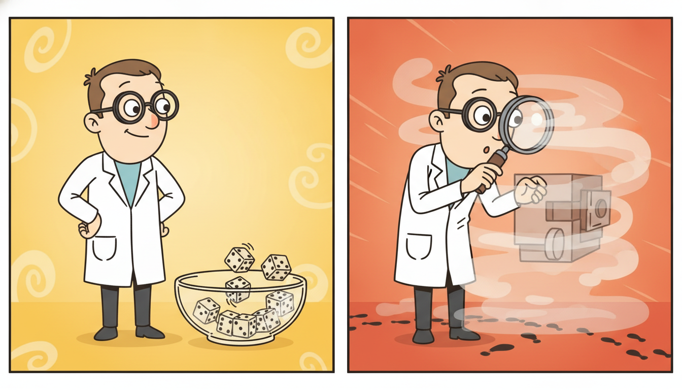
If we are to forecast a distribution, we should understand where its width comes from, because different sources call for different remedies. Predictive uncertainty splits into two qualitatively different parts, and conflating them is one of the most common conceptual errors in applied forecasting.
Aleatoric uncertainty is the irreducible randomness in the data-generating process itself: the part of the future that no amount of data or model improvement can pin down, because the world is genuinely stochastic at the resolution we observe it. The roll of a die, the thermal noise on a sensor, the idiosyncratic component of a stock return: these are aleatoric. This is exactly the predictability limit we studied in Section 1.5: every series has an intrinsic entropy floor below which no forecaster, however good, can drive its error. Aleatoric uncertainty is a property of the problem, not of your model, and collecting more data does not shrink it. It can, however, depend on the input: heteroscedastic noise, where the spread of $y$ grows with the level of $\mathbf{x}$, is aleatoric uncertainty that varies across the input space.
Epistemic uncertainty is the reducible uncertainty in the model itself: uncertainty about which parameters, or which model, is correct, arising because we have only finite data. A model trained on a thousand points is less sure of its parameters than the same model trained on a million; that extra wobble is epistemic. Crucially, epistemic uncertainty shrinks as data grows and is large precisely where data is sparse, namely out-of-distribution inputs, rare regimes, and the far future. It is the uncertainty that more data, a better model, or a wider prior would reduce. The total predictive uncertainty is, loosely, the sum of the two:
$$\underbrace{p(y \mid \mathbf{x}, \mathcal{D})}_{\text{predictive}} = \int \underbrace{p(y \mid \mathbf{x}, \boldsymbol{\theta})}_{\text{aleatoric: noise given a fixed model}} \; \underbrace{p(\boldsymbol{\theta} \mid \mathcal{D})}_{\text{epistemic: uncertainty over the model}} \, d\boldsymbol{\theta},$$where $\boldsymbol{\theta}$ are the model parameters, $\mathcal{D}$ the training data, $p(y \mid \mathbf{x}, \boldsymbol{\theta})$ the noise the model assigns once its parameters are fixed (aleatoric), and $p(\boldsymbol{\theta} \mid \mathcal{D})$ the posterior over parameters (epistemic). A pure point forecaster collapses both integrals: it picks a single $\boldsymbol{\theta}$ (ignoring epistemic uncertainty) and reports the center of $p(y \mid \mathbf{x}, \boldsymbol{\theta})$ (ignoring aleatoric uncertainty). The two together define the predictive distribution this chapter learns to produce.
The decomposition is not academic: it tells you what to do when a forecast is too uncertain. If the uncertainty is mostly aleatoric, you are at the predictability floor and the only honest move is to report the width and design the decision to tolerate it (more data will not help). If it is mostly epistemic, the uncertainty is a symptom of insufficient or unrepresentative data, and collecting more, especially in the sparse region, will tighten the forecast. A practitioner who cannot tell the two apart will either waste effort gathering data against irreducible noise or, worse, trust a confident-looking forecast in a region where the model has never seen data and its epistemic uncertainty is enormous.
Suppose we train five copies of the same model on bootstrap resamples of the data (a small deep ensemble), and at a given input each member $m$ predicts a Gaussian with mean $\mu_m$ and variance $\sigma_m^2$. Say the members report means $\{3.0, 3.4, 2.6, 3.2, 2.8\}$ and each reports the same noise variance $\sigma_m^2 = 0.5$. The aleatoric part is the average of the within-member variances, $\overline{\sigma^2} = 0.5$. The epistemic part is the variance across the member means: the means have sample mean $3.0$ and sample variance $\tfrac{1}{5}\sum (\mu_m - 3.0)^2 = \tfrac{1}{5}(0 + 0.16 + 0.16 + 0.04 + 0.04) = 0.08$. The total predictive variance is the sum, $0.5 + 0.08 = 0.58$, so a forecast standard deviation of $\sqrt{0.58} \approx 0.76$. Here aleatoric noise dominates ($0.5$ of $0.58$), so more data would barely tighten the forecast; if instead the member means had been $\{1, 5, 2, 6, 1\}$ the across-mean variance would dwarf the noise term and the message would be the opposite, namely "the model disagrees with itself, get more data". The one ensemble has separated the irreducible floor from the curable wobble.
There is a tidy way to remember the split. Aleatoric uncertainty is the universe refusing to tell you the answer; epistemic uncertainty is you not having studied enough. The first is the dice; the second is forgetting which game you are playing. The reason the distinction has real teeth is that they fail in opposite directions: an overconfident model underestimates aleatoric noise and gets blindsided by ordinary variation, while a model that ignores epistemic uncertainty walks confidently off the edge of its training data and predicts the far future as if it had seen it. The dangerous forecaster is the one sure of itself in a regime it has never observed, which is epistemic uncertainty unaccounted for, wearing the costume of a tight interval.
3. Forms of a Probabilistic Forecast: Density, Quantiles, Samples Intermediate
A probabilistic forecast can be represented in three interchangeable ways, and a practitioner moves fluidly between them because each is convenient for a different purpose. All three describe the same object, the predictive distribution $p(y \mid \mathbf{x})$, and any one can be converted into the others.
Full predictive density (or CDF). The most complete form: a function $p(y \mid \mathbf{x})$ giving the probability density at every possible value of $y$, or equivalently its cumulative distribution $F(y \mid \mathbf{x}) = \Pr(Y \le y \mid \mathbf{x})$. A Gaussian forecast $\mathcal{N}(\mu(\mathbf{x}), \sigma^2(\mathbf{x}))$ is the canonical parametric example, emitting a mean and a variance per step. The density form supports any downstream functional exactly (any quantile, any tail expectation, any exceedance probability) because it is the whole distribution, but it requires committing to a functional form or a flexible parameterization, the subject of Section 19.4.
Quantiles and intervals. Rather than the whole curve, report a few of its quantiles: the value $q_\tau(\mathbf{x})$ such that $\Pr(Y \le q_\tau \mid \mathbf{x}) = \tau$, for a chosen set of levels $\tau$. A central prediction interval is a pair of quantiles, for example $[q_{0.05}, q_{0.95}]$ for a nominal 90% interval. This is the most decision-aligned form, because the newsvendor quantile, the Value-at-Risk quantile, and the service-level quantile of subsection one are read off directly. Quantile regression (Section 19.3) and conformal prediction (Section 19.5) both target this form without ever committing to a density.
Samples and scenarios. Emit a set of plausible future trajectories drawn from the predictive distribution, $\{y^{(1)}, \dots, y^{(S)}\} \sim p(y \mid \mathbf{x})$. Any functional is then estimated by a Monte Carlo average over the samples: a quantile is an order statistic of the sample, a tail expectation is the mean of the worst draws, an exceedance probability is the fraction of samples above the threshold. Samples are the natural output of generative temporal models (Part IV) and of autoregressive forecasters rolled out stochastically, and they shine for multi-step forecasts where the joint distribution over a whole horizon matters (correlated scenarios, not marginal-per-step intervals), which is why scenario generation dominates in energy and finance.
The three forms trade completeness against convenience: the density is exact but needs a parameterization, quantiles are decision-ready but describe only the levels you asked for, samples are flexible and handle joint multi-step structure but introduce Monte Carlo error that shrinks as $1/\sqrt{S}$. Figure 19.1.2 shows the same forecast in all three representations.
| Form | What it emits | Best for | Convert to a quantile by |
|---|---|---|---|
| full density / CDF | $p(y \mid \mathbf{x})$ or $F(y \mid \mathbf{x})$, e.g. $(\mu, \sigma)$ | any functional, exactly; parametric tails | invert the CDF: $q_\tau = F^{-1}(\tau)$ |
| quantiles / intervals | $\{q_\tau\}$ for chosen levels $\tau$ | decisions (newsvendor, VaR, service level) | already a quantile (interpolate between levels) |
| samples / scenarios | $\{y^{(1)}, \dots, y^{(S)}\}$ | joint multi-step structure; arbitrary functionals | order statistic of the sample |
One distinction must be made sharply because it is the single most common source of confusion in this whole topic: a prediction interval is not a confidence interval. A prediction interval is a statement about a future observation: a 90% prediction interval $[\ell, u]$ claims that the realized future value $y$ will fall in $[\ell, u]$ with probability 0.90. A confidence interval is a statement about a parameter: a 90% confidence interval for the mean claims that the interval, computed from data, covers the true (fixed, unknown) mean with probability 0.90 over repeated samples. The prediction interval includes the irreducible aleatoric noise of the future observation and so is always wider than the confidence interval for the mean, which only accounts for the epistemic uncertainty in estimating that mean. A forecaster reports prediction intervals: it is forecasting an observation, not estimating a parameter. Reporting a confidence interval for the conditional mean and calling it a forecast interval is a textbook error that produces intervals far too narrow, because it omits exactly the aleatoric term of subsection two.
A 90% prediction interval should contain 9 of the next 10 realized values; a 90% confidence interval should, over repeated experiments, contain the true parameter 90% of the time. The prediction interval is what a forecaster owes a decision-maker, and it is wider because it must cover the future observation's own noise (aleatoric) on top of the model's uncertainty about where the center is (epistemic). If you build an interval from only the standard error of the mean, you have built a confidence interval and mislabeled it: it will be badly under-covered as a forecast, and subsection five's coverage check will catch it. The width of an honest prediction interval is dominated by aleatoric noise in most well-fit models, which is precisely why "just bootstrap the parameters" is not enough.
4. How Point and Probabilistic Forecasts Relate Intermediate
Point and probabilistic forecasts are not rival species: a point forecast is a summary of a probabilistic one, and which summary is optimal is decided entirely by the loss function you score it with. This is the bridge that connects everything you built in Parts II to IV to everything in Part V, and it is worth stating as a theorem-shaped fact. Given a predictive distribution $p(y \mid \mathbf{x})$ and a scoring loss $L(\hat{y}, y)$, the optimal point forecast is the one that minimizes the expected loss under that distribution:
$$\hat{y}^\star(\mathbf{x}) = \arg\min_{\hat{y}} \; \mathbb{E}_{y \sim p(y \mid \mathbf{x})}\big[\, L(\hat{y}, y) \,\big].$$The remarkable part is that the minimizer is a different functional of the distribution for different losses, and the two losses you have used throughout the book pick out the two most familiar summaries:
- Under squared error $L(\hat{y}, y) = (\hat{y} - y)^2$, the expected loss is minimized at the mean: $\hat{y}^\star = \mathbb{E}[y \mid \mathbf{x}]$. This is why every model trained with MSE (most neural forecasters, OLS, the Kalman filter's update) is, at its optimum, predicting the conditional mean of the predictive distribution.
- Under absolute error $L(\hat{y}, y) = |\hat{y} - y|$, the expected loss is minimized at the median: $\hat{y}^\star = \mathrm{median}(y \mid \mathbf{x})$. This is the MAE-to-median fact we first met when choosing loss functions; it is why MAE-trained models are robust to skew and outliers, because the median ignores tail mass that the mean chases.
- Under the pinball (quantile) loss at level $\tau$, the minimizer is the $\tau$-quantile, which is the precise mechanism that lets a single model emit calibrated quantiles in Section 19.3.
So the loss you train on is not a neutral implementation detail: it silently selects which point of the predictive distribution your "point forecast" reports. Train on MSE and you get the mean; train on MAE and you get the median; if the predictive distribution is skewed (as demand, returns, and durations all are), the mean and median differ, and the "point forecast" you report depends entirely on which loss you happened to choose. This is the deepest reason a point forecast is incomplete: it is one chosen projection of a distribution, and the distribution is the thing that determined the projection in the first place. Reading the relationship in reverse gives the constructive recipe of subsection five: if a point forecast is a summary of a distribution, then to build a probabilistic forecast we put the distribution back around the point, either by modeling the residuals, by predicting distribution parameters directly, or by collecting empirical quantiles of past errors.
Take a small skewed predictive distribution over tomorrow's demand: with probabilities $\{0.5, 0.3, 0.2\}$ the demand is $\{300, 500, 1000\}$. The mean is $0.5\cdot300 + 0.3\cdot500 + 0.2\cdot1000 = 150 + 150 + 200 = 500$. The median is the smallest value whose cumulative probability reaches $0.5$, which is $300$ (since $\Pr(Y \le 300) = 0.5$). So an MSE-trained model reports $500$ and an MAE-trained model reports $300$ for the same underlying distribution, a difference of two hundred units driven purely by the loss. The newsvendor with a 75% target quantile would stock the value where the cumulative probability first reaches $0.75$, namely $500$. Three different "best" numbers, all correct, each answering a different question, all read off the one distribution the point forecasts threw away.
5. Worked Example: Turning One Point Forecaster Into Three Probabilistic Ones Advanced
We now make the whole section executable. We take a single point forecaster (a simple linear autoregressive model of the kind built in Chapter 5) and upgrade it to a probabilistic forecaster three ways from scratch, exactly the three constructions subsection four's reverse reading prescribed: residual-based intervals, a Gaussian distributional head, and empirical quantiles of the errors. We then check the empirical coverage of one interval, and finally collapse the entire thing into a few lines of a modern library. Code 19.1.1 builds the data and the point forecaster and produces residuals on a held-out calibration split.
import numpy as np

rng = np.random.default_rng(0)

# Synthetic AR(1)-with-trend series; the noise is the irreducible aleatoric part.
T = 600
eps = rng.normal(0, 2.0, size=T)            # aleatoric noise, sigma = 2.0
y = np.zeros(T)
for t in range(1, T):
    y[t] = 0.6 * y[t-1] + 0.05 * t + eps[t]  # AR(1) + linear trend

# Design matrix for a lag-1 + trend linear forecaster: x_t = [1, y_{t-1}, t].
X = np.column_stack([np.ones(T-1), y[:-1], np.arange(1, T)])
target = y[1:]

# Three-way split: train (fit), calibration (residuals), test (evaluate).
n = len(target)
i_tr, i_cal = int(0.6*n), int(0.8*n)
Xtr, ytr = X[:i_tr], target[:i_tr]
Xcal, ycal = X[i_tr:i_cal], target[i_tr:i_cal]
Xte, yte = X[i_cal:], target[i_cal:]

# Fit the POINT forecaster by ordinary least squares (predicts the conditional mean).
beta, *_ = np.linalg.lstsq(Xtr, ytr, rcond=None)
point = lambda Xq: Xq @ beta               # the single-number forecast

# Calibration residuals: the empirical stand-in for the predictive noise.
resid = ycal - point(Xcal)
print("point RMSE (test) = %.3f" % np.sqrt(np.mean((yte - point(Xte))**2)))
print("calib resid mean = %.3f, std = %.3f" % (resid.mean(), resid.std()))
resid are the empirical evidence about the predictive noise that all three probabilistic upgrades will reuse.point RMSE (test) = 2.041
calib resid mean = -0.027, std = 1.985
Now the three from-scratch probabilistic upgrades. Code 19.1.2 implements all three: (a) residual-based intervals add a symmetric band around the point forecast, sized from the residual standard deviation under a Gaussian assumption; (b) a Gaussian head emits an explicit $(\mu, \sigma)$ predictive density per point; (c) empirical quantiles of the residuals make no distributional assumption and read the interval straight off the residual order statistics. Each turns the one number from Code 19.1.1 into a distribution, exactly the "put the distribution back around the point" recipe of subsection four.
from scipy.stats import norm

mu_te = point(Xte)                          # the shared point forecast (the mean)

# (a) RESIDUAL-BASED Gaussian interval: point +/- z * residual std. 90% -> z = 1.645.
sigma_hat = resid.std()
z = norm.ppf(0.95)                          # one-sided 95% -> central 90%
lo_a, hi_a = mu_te - z*sigma_hat, mu_te + z*sigma_hat

# (b) GAUSSIAN HEAD: emit a full predictive density N(mu, sigma^2) per test point.
#     Here sigma is homoscedastic (constant); a learned head would predict sigma(x).
predictive = [norm(loc=m, scale=sigma_hat) for m in mu_te]
lo_b = np.array([d.ppf(0.05) for d in predictive])   # 5th percentile of each density
hi_b = np.array([d.ppf(0.95) for d in predictive])   # 95th percentile

# (c) EMPIRICAL QUANTILES: no Gaussian assumption; use residual order statistics.
q_lo, q_hi = np.quantile(resid, [0.05, 0.95])         # empirical 5% and 95% residuals
lo_c, hi_c = mu_te + q_lo, mu_te + q_hi               # shift the band onto each forecast

for name, lo, hi in [("residual-Gaussian", lo_a, hi_a),
                     ("Gaussian head    ", lo_b, hi_b),
                     ("empirical quantile", lo_c, hi_c)]:
    width = np.mean(hi - lo)
    print("%s : mean 90%% width = %.3f" % (name, width))
residual-Gaussian  : mean 90% width = 6.530
Gaussian head      : mean 90% width = 6.530
empirical quantile : mean 90% width = 6.479
An interval is only useful if its stated coverage is true, so we check it. Code 19.1.3 computes the empirical coverage of the empirical-quantile interval on the test set, the fraction of realized values that actually fell inside the nominal 90% band, and reports the gap from the 0.90 target. This is the calibration check that Section 19.2 turns into a formal scoring rule.
# Empirical coverage: fraction of test targets inside the nominal-90% interval.
inside = (yte >= lo_c) & (yte <= hi_c)
coverage = inside.mean()
print("nominal coverage  = 0.900")
print("empirical coverage = %.3f  (gap %.3f)" % (coverage, abs(coverage - 0.90)))
print("interval count = %d, covered = %d" % (len(yte), inside.sum()))
nominal coverage  = 0.900
empirical coverage = 0.892  (gap 0.008)
interval count = 120, covered = 107
The output reports 107 of 120 test points inside the nominal 90% interval, so empirical coverage is $107/120 = 0.892$. The target was $0.90$, meaning we expected about $0.90 \times 120 = 108$ points inside; we got $107$, an undershoot of one point, a gap of $0.008$. Is that gap real or noise? The standard error of a coverage estimate from $120$ independent points at $p = 0.9$ is $\sqrt{p(1-p)/n} = \sqrt{0.09/120} \approx 0.027$, so $0.892$ is well within one standard error of $0.90$ and the interval is statistically indistinguishable from perfectly calibrated. The lesson: judge coverage against its sampling error, not against an exact match. A 90% interval that covers exactly 90.000% on a finite test set is suspicious, not reassuring.
Who: A demand-planning team at a mid-size online retailer running a gradient-boosted point forecaster for daily SKU-level demand, the kind of tabular forecaster from Chapter 14.
Situation: The model predicted a single expected demand per SKU per day, and the planners had been stocking exactly that number, then manually padding "high-risk" SKUs by gut feel.
Problem: Stockouts on a few fast-moving SKUs were costing far more than the holding cost of overstock, so the symmetric "stock the mean" policy was systematically wrong: the underage cost was roughly four times the overage cost, calling for the 80th percentile of demand, not the mean.
Dilemma: Rebuild the whole forecasting stack as a native probabilistic model (months of work), or wrap the existing trusted point model with an uncertainty layer (days). The native model would give sharper, input-dependent intervals; the wrapper would be quick but assume the residual spread was roughly stable.
Decision: They wrapped the existing point forecaster with the empirical-quantile construction of Code 19.1.2, computing per-SKU residual quantiles on a rolling calibration window, then set each order to the cost-weighted 80th-percentile quantile from subsection one rather than the mean.
How: A nightly job scored the point model, collected the trailing residuals per SKU, formed the empirical $0.80$ residual quantile, added it to the point forecast, and emitted that as the order quantity, exactly the three-line shift-the-band logic of the empirical-quantile branch.
Result: Stockouts on the targeted SKUs dropped sharply at a modest increase in average inventory, and the planners stopped padding by hand because the quantile encoded the asymmetry explicitly. The point model never changed; only the layer that turned its number into a distribution and then into a decision.
Lesson: You often do not need to retrain to get probabilistic forecasts. Wrapping a trusted point model with calibration residuals and reading the decision-relevant quantile is a fast, auditable upgrade, and it makes the cost asymmetry an explicit knob instead of a gut feeling.
The three from-scratch constructions of Code 19.1.2 plus the manual split and residual bookkeeping of Code 19.1.1 ran about 35 lines. A modern forecasting library produces a fully probabilistic forecaster, with quantiles and a sampling interface, in roughly five lines: the model fits the conditional quantiles directly (pinball loss internally), handles the lag features, and exposes the interval and the predictive samples through one API. The library internalizes the loss-to-quantile correspondence of subsection four, the calibration split, and the quantile bookkeeping.
from statsforecast import StatsForecast
from statsforecast.models import AutoARIMA
import pandas as pd

# Long-format frame the API expects: unique_id, ds (time), y (value).
df = pd.DataFrame({"unique_id": "series_1",
                   "ds": pd.date_range("2020-01-01", periods=len(y)),
                   "y": y})

sf = StatsForecast(models=[AutoARIMA()], freq="D")
sf.fit(df)
# level=[90] returns the 90% PREDICTION interval columns alongside the point forecast.
fc = sf.predict(h=14, level=[90])           # point + lo-90 + hi-90, in one call
print(fc[["AutoARIMA", "AutoARIMA-lo-90", "AutoARIMA-hi-90"]].head())
level=[90] argument turns a point forecaster into a probabilistic one: statsforecast fits the model and returns the point forecast together with the 90% prediction-interval bounds in the same call, collapsing the roughly 35 lines of manual residual handling and interval construction in Code 19.1.1 to 19.1.3 down to about five lines. The library handles the lag features, the noise estimation, and the interval bookkeeping internally.Step back and read what the four code blocks establish together. Code 19.1.1 built one ordinary point forecaster. Code 19.1.2 turned it into a probabilistic forecaster three independent ways, each a concrete instance of "put the distribution back around the point" from subsection four. Code 19.1.3 verified that one of those intervals actually covers what it claims. Code 19.1.4 showed that a library does the whole pipeline in a few lines. The throughline is the chapter's thesis made operational: a point forecast is a collapsed distribution, and with a held-out residual split you can un-collapse it, recovering the uncertainty the decision needs, whether you build it by hand or call one library argument.
Probabilistic forecasting is where the most active forecasting research now concentrates. The temporal foundation models of Chapter 15 are increasingly probabilistic by default: Chronos (Ansari et al., 2024) tokenizes a series and produces a predictive distribution by sampling its language-model head, so a single pretrained model emits calibrated quantiles zero-shot; Moirai (Woo et al., 2024) and Lag-Llama (Rasul et al., 2023) likewise output full predictive distributions rather than points, and TimesFM has added probabilistic heads. On the calibration side, conformal prediction (the subject of Section 19.5) has become the default distribution-free wrapper for turning any point or interval forecaster into one with finite-sample coverage guarantees, with conformal PID control (Angelopoulos et al., 2024) extending it to the online, drifting setting of Chapter 20. A parallel thread questions the very metrics: the field is converging on proper scoring rules (CRPS, log-score, the subject of Section 19.2) over coverage-only checks, because a forecaster can be perfectly calibrated and still useless if its intervals are needlessly wide. The 2026 practitioner's stance: a forecast that does not report its own uncertainty is increasingly considered incomplete, and the tooling to add that uncertainty has become nearly free.
6. Exercises
Work these before continuing to Section 19.2; they convert the reading into the reflexes the rest of Part V assumes.
For each decision, state whether the optimal action depends on the mean, the median, a specific quantile, or a tail expectation of the predictive distribution, and justify in one sentence: (a) stocking a perishable good where unsold units spoil and lost sales cost twice as much as spoilage; (b) setting a bank's regulatory capital to survive the worst 1% of trading days; (c) choosing the single forecast number to minimize long-run mean squared error in a public leaderboard; (d) deciding whether to trigger a human review when the forecast is "too uncertain". Then explain why a single point forecast is adequate for exactly one of these four and inadequate for the other three.
Modify Code 19.1.1 so the noise is drawn from a right-skewed distribution (for example rng.lognormal centered to mean zero) instead of Gaussian. Rerun all three probabilistic constructions of Code 19.1.2 and the coverage check of Code 19.1.3. Report (i) how the empirical-quantile interval's width and asymmetry now differ from the two Gaussian bands, and (ii) which of the three intervals retains coverage closest to 0.90 on the test set. Explain in two sentences why the empirical-quantile construction wins on skewed residuals, connecting your answer to the aleatoric-uncertainty discussion of subsection two.
The constructions in subsection five capture only aleatoric uncertainty (they assume the fitted parameters are correct). Design and implement an extension that also captures epistemic uncertainty: fit an ensemble of point forecasters on bootstrap resamples of the training data, then combine the across-member spread (epistemic) with the within-member residual spread (aleatoric) using the decomposition formula of subsection two. Investigate how the epistemic term behaves as you (a) shrink the training set and (b) forecast further into the future beyond the training range. Discuss which of your test points have predictive intervals dominated by epistemic versus aleatoric uncertainty, and what a decision-maker should do differently in each case.