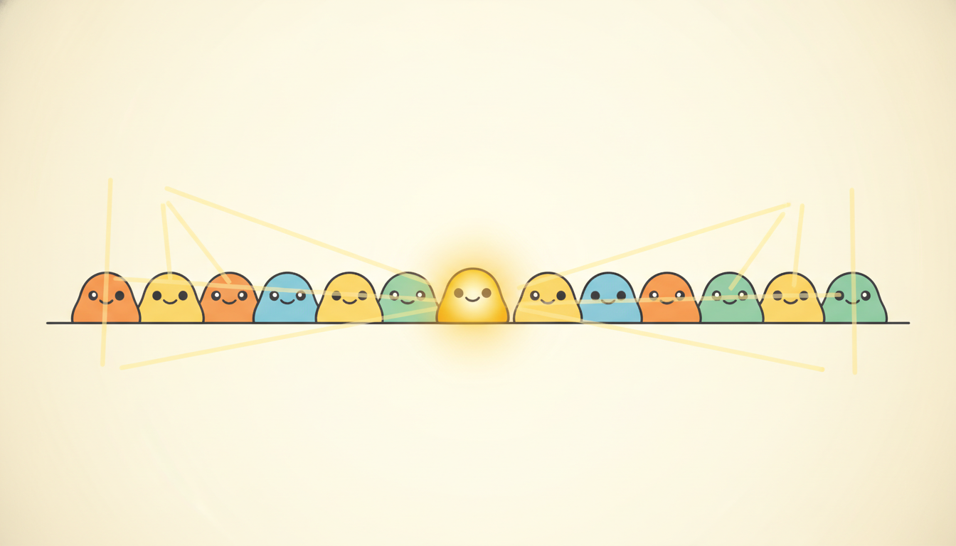
"I do not pass a message hand to hand down a line of clerks, hoping it survives a thousand whispered relays. I stand in the middle of the room and look at everyone at once, weigh whose words matter for the question I was asked, and take a weighted average of the answers. It is exhausting, the looking costs me the square of the crowd, but nothing reaches me secondhand and nothing fades on the way."
An Attention Head Looking Everywhere at Once
Self-attention replaces the recurrence $\mathbf{h}_t = f(\mathbf{h}_{t-1}, \mathbf{x}_t)$ with a single, parallel operation in which every position computes a content-based, data-dependent weighted average over every other position. Each position emits a query, every position offers a key and a value; the query scores itself against all keys by a scaled dot product, those scores become a softmax distribution, and the output is that distribution's weighted sum of values. The one equation $\operatorname{Attention}(\mathbf{Q},\mathbf{K},\mathbf{V}) = \operatorname{softmax}\!\big(\mathbf{Q}\mathbf{K}^\top/\sqrt{d}\big)\mathbf{V}$ carries the whole idea. Because the average is over all positions directly, there is no fixed-width hidden state to bottleneck information and no long chain of Jacobians to vanish through: any position can reach any other in one step. The price is quadratic: scoring every pair costs $O(L^2 d)$ time and memory, in contrast to the $O(L)$ sequential recurrence of Section 10.4. Multiple heads run this operation in several learned subspaces at once, so the layer can attend to different relations in parallel; a causal mask forbids attending to the future, which is what makes self-attention safe for forecasting. This section motivates the mechanism from the seq2seq bottleneck, derives scaled dot-product and multi-head attention with full math, implements both from scratch in torch and via nn.MultiheadAttention, and computes one attention weight by hand. It is the foundation for the Transformer block of Section 12.2 and every architecture in the rest of this chapter.
In Section 10.4 we built sequence-to-sequence models: an encoder RNN compresses an input sequence into a hidden state, and a decoder RNN unrolls that state into an output sequence. We ended that section on a warning. The encoder must funnel the entire input, however long, through a single fixed-width vector before the decoder sees any of it, and that vector is the bottleneck through which all information must pass. This section removes the bottleneck entirely. Instead of forcing every input position to be summarized into one state and then read back out, we let each position of the sequence attend directly to every other position, reading exactly what it needs from wherever it lives, with no intermediate compression. That single change, direct all-to-all access in place of a relayed summary, is the whole of self-attention, and it is the architectural idea on which the Transformer, and most of modern temporal deep learning, is built. We use the unified notation of Appendix A throughout: $\mathbf{x}_t$ the input at position $t$, $L$ the sequence length, $d$ the model width.
Why does this idea deserve a chapter rather than a footnote to the RNN? Because it changes the two quantities that govern whether a sequence model can learn long-range structure: the path length over which information travels, and the degree to which computation can be parallelized. In a recurrence, information from position $1$ reaches position $L$ only by passing through $L-1$ intermediate states, a path whose length grows with the sequence and along which gradients vanish (Section 9.4). In self-attention that path length is one: every position is one weighted average away from every other, independent of how far apart they sit. And because the average for each position is computed independently, the whole layer runs in parallel across positions rather than stepping through time. The cost of buying constant path length and full parallelism is the quadratic interaction we examine in subsection four, and the rest of Part III can be read as a sustained negotiation between that quadratic cost and the linear recurrence it replaced.
The four competencies this section installs are these: to explain the seq2seq bottleneck and why direct attention dissolves it; to read and derive scaled dot-product attention as a learned, content-based, data-dependent average, and to say why the $\sqrt{d}$ scaling is there; to describe multi-head attention, the self-versus-cross distinction, and causal masking for leak-free forecasting; and to implement attention from scratch and verify it against the library primitive. These are load-bearing for the Transformer architecture of Section 12.2, the positional encodings of Section 12.3, and the efficient-attention variants of Section 12.5.
1. The Seq2Seq Bottleneck and the Idea of Direct Attention Beginner
Recall the encoder-decoder picture from Section 10.4. An encoder RNN reads the input sequence $\mathbf{x}_1, \dots, \mathbf{x}_L$ one step at a time and, after the last step, hands the decoder a single context vector $\mathbf{c} = \mathbf{h}_L$, the final hidden state. The decoder then generates its output sequence conditioned only on $\mathbf{c}$. Everything the model knows about a possibly very long input has been squeezed into one fixed-width vector, and the decoder must reconstruct whatever it needs from that one summary. This is the information bottleneck: the context vector has a fixed dimension regardless of input length, so as sequences grow, more and more must be crammed into the same number of numbers, and early positions in particular are overwritten by later ones as the encoder state is updated step by step.
The empirical signature of the bottleneck is sharp. Encoder-decoder models without attention degrade badly as input length grows, and they degrade most on information from the start of the sequence, exactly the positions that have been most diluted by the time the encoder finishes. The first repair, due to Bahdanau and colleagues in 2015, was to let the decoder, at each output step, look back over all the encoder states $\mathbf{h}_1, \dots, \mathbf{h}_L$ and take a weighted average of them, with the weights computed from how relevant each input position is to the current decoding step. The fixed context vector becomes a dynamic, per-step context, and the bottleneck is gone: information no longer has to survive being compressed into one vector, because the decoder can reach back to any encoder position directly.
Self-attention is the radical generalization of that repair. The Bahdanau mechanism let a decoder attend to an encoder. Self-attention asks: why not let a sequence attend to itself, with every position building its representation as a weighted average over every position of the same sequence, and dispense with the recurrence altogether? If position $t$ can read directly from every other position, the encoder no longer needs to carry information forward step by step in a hidden state at all. The recurrence, with its fixed-width state and its sequential path, was only ever a mechanism for moving information across time; direct attention moves it in one hop. Figure 12.1.1 contrasts the relayed path of the recurrence with the direct all-to-all access of self-attention.
Two consequences follow immediately and frame the rest of the section. First, because there is no recurrence, the operation has no inherent notion of order: a self-attention layer treats its input as a set, and order must be injected separately by the positional encodings of Section 12.3. Second, because every position is averaged against every other, the work scales with the number of pairs, $L^2$, the quadratic cost that subsection four weighs against the recurrence's linear pass. The mechanism trades a long, sequential, fading path for a short, parallel, expensive one, and that trade is the central economic fact of modern sequence modeling.
The recurrence moves information across time by relaying it through a chain of fixed-width hidden states, so distant positions are far apart (long path) and early information is diluted (fixed-width bottleneck). Self-attention moves information by letting each position take a weighted average directly over all positions, so every position is one hop from every other and nothing is compressed into a single carried vector. You buy constant path length and full parallelism; you pay with quadratic interaction and the loss of any built-in sense of order. Everything else in this chapter elaborates that one exchange.
2. Queries, Keys, Values, and Scaled Dot-Product Attention Intermediate
Make the idea precise. We are given a sequence of $L$ vectors, stacked as rows of a matrix $\mathbf{X} \in \mathbb{R}^{L \times d}$. We want each position to produce an output that is a weighted average over all positions, where the weights depend on the content of the positions, not their indices. The mechanism uses three learned linear projections of the input, named by an analogy to a soft dictionary lookup: a query says what a position is looking for, a key says what a position offers, and a value is what a position actually contributes once it is selected. With projection matrices $\mathbf{W}^Q, \mathbf{W}^K \in \mathbb{R}^{d \times d_k}$ and $\mathbf{W}^V \in \mathbb{R}^{d \times d_v}$,
$$\mathbf{Q} = \mathbf{X}\mathbf{W}^Q, \qquad \mathbf{K} = \mathbf{X}\mathbf{W}^K, \qquad \mathbf{V} = \mathbf{X}\mathbf{W}^V,$$so $\mathbf{Q} \in \mathbb{R}^{L \times d_k}$ holds one query per position, and likewise $\mathbf{K}$ and $\mathbf{V}$. The relevance of position $j$ to position $i$ is measured by the dot product of query $i$ with key $j$, $\mathbf{q}_i^\top \mathbf{k}_j$, a scalar that is large when the query and key point in similar directions. Collecting all pairs at once, $\mathbf{Q}\mathbf{K}^\top \in \mathbb{R}^{L \times L}$ is the matrix of raw scores, entry $(i,j)$ being how much position $i$ should attend to position $j$. We turn each row of scores into a probability distribution with a softmax, and the output at each position is that distribution's weighted average of the value vectors. The complete operation is scaled dot-product attention:
$$\operatorname{Attention}(\mathbf{Q}, \mathbf{K}, \mathbf{V}) = \operatorname{softmax}\!\left(\frac{\mathbf{Q}\mathbf{K}^\top}{\sqrt{d_k}}\right)\mathbf{V}.$$Read it left to right as a four-step pipeline. The product $\mathbf{Q}\mathbf{K}^\top$ scores every query against every key. Dividing by $\sqrt{d_k}$ rescales the scores. The row-wise softmax converts each row of scores into nonnegative weights that sum to one, the attention weights $\mathbf{A} \in \mathbb{R}^{L \times L}$ with $A_{ij} \ge 0$ and $\sum_j A_{ij} = 1$. Multiplying by $\mathbf{V}$ replaces each position by the $\mathbf{A}$-weighted average of all value vectors. The output for position $i$ is $\sum_j A_{ij}\,\mathbf{v}_j$, a convex combination of values whose mixing coefficients were chosen by content.
The single most useful way to hold the operation in mind is this: an attention layer computes, for each position, a learned, content-based, data-dependent average over the sequence. It is an average because the weights are nonnegative and sum to one. It is content-based because the weights come from how the query and keys point, not from fixed positions. It is data-dependent because the same layer produces entirely different weights for different inputs, in contrast to a convolution whose mixing weights are fixed once trained. And it is learned because $\mathbf{W}^Q, \mathbf{W}^K, \mathbf{W}^V$ are trained by gradient descent to make the right things attend to the right things. This is the precise sense in which attention generalizes the fixed weighted averages of a moving-average filter (Chapter 5) into a weighting that the data itself chooses at run time.
Why divide by $\sqrt{d_k}$? Suppose the entries of the query and key vectors are independent with zero mean and unit variance. Then each dot product $\mathbf{q}_i^\top \mathbf{k}_j = \sum_{m=1}^{d_k} q_{im} k_{jm}$ is a sum of $d_k$ independent zero-mean unit-variance products, so its variance is $d_k$ and its typical magnitude grows like $\sqrt{d_k}$. Feed scores of magnitude $\sqrt{d_k}$ into a softmax and, for the large widths used in practice ($d_k$ of 64 or more), the softmax saturates: one entry dominates, the distribution collapses toward a one-hot spike, and its gradient with respect to the scores becomes vanishingly small, so the layer cannot learn. Dividing by $\sqrt{d_k}$ rescales the scores back to unit variance, keeping the softmax in its responsive regime where gradients flow. The scaling is not cosmetic; without it, attention with wide heads trains poorly or not at all.
Take a query position with query vector $\mathbf{q} = (1, 0)$ ($d_k = 2$) attending over three positions whose keys are $\mathbf{k}_1 = (1, 0)$, $\mathbf{k}_2 = (0, 1)$, $\mathbf{k}_3 = (1, 1)$. The raw scores are the dot products $\mathbf{q}^\top\mathbf{k}_1 = 1$, $\mathbf{q}^\top\mathbf{k}_2 = 0$, $\mathbf{q}^\top\mathbf{k}_3 = 1$. Scale by $\sqrt{d_k} = \sqrt{2} \approx 1.414$: the scaled scores are $0.707, 0, 0.707$. Exponentiate: $e^{0.707} \approx 2.028$, $e^{0} = 1$, $e^{0.707} \approx 2.028$, summing to $5.056$. The attention weights are therefore $A_1 = 2.028/5.056 \approx 0.401$, $A_2 = 1/5.056 \approx 0.198$, $A_3 = 0.401$. The query splits its attention roughly $40/20/40$, favoring positions 1 and 3 whose keys align with it and discounting position 2 whose key is orthogonal. If the values were $\mathbf{v}_1 = (10,0)$, $\mathbf{v}_2 = (0,10)$, $\mathbf{v}_3 = (5,5)$, the output is $0.401(10,0) + 0.198(0,10) + 0.401(5,5) = (6.02, 3.99)$. Notice the effect of the scaling: had we skipped the $\sqrt{2}$ divisor, the scores $1,0,1$ would have given a sharper $42/16/42$ split; with wide heads the unscaled sharpening is far more extreme and is exactly what the divisor tames.
It is worth naming what attention is not, to forestall a common misreading. The attention weight $A_{ij}$ is not a probability that position $j$ caused or determined position $i$; it is a mixing coefficient in a soft, differentiable lookup. The whole construction is differentiable precisely because the hard "pick the most relevant position" of a discrete dictionary lookup has been softened into "take a weighted blend of all positions", and the softmax is what does the softening. That differentiability is what lets the projections $\mathbf{W}^Q, \mathbf{W}^K, \mathbf{W}^V$ be learned end to end by the same backpropagation we built in Section 9.3, now flowing through the softmax and the two matrix products rather than through a recurrence.
Three projections turn each position into a query (what it seeks), a key (what it advertises), and a value (what it carries). The query-key dot products, scaled by $\sqrt{d_k}$ and softmaxed, are the addressing weights; the output is those weights' average of the values. The $\sqrt{d_k}$ scaling keeps the softmax responsive at large width. Because every step is differentiable, the projections learn, by ordinary gradient descent, to route each position's query to the keys that carry the information it needs. Hold onto the one-line summary: $\operatorname{Attention}(\mathbf{Q},\mathbf{K},\mathbf{V}) = \operatorname{softmax}(\mathbf{Q}\mathbf{K}^\top/\sqrt{d_k})\mathbf{V}$ is a learned, content-based, data-dependent weighted average over the sequence.
3. Multiple Heads, Self versus Cross, and Causal Masking Intermediate
A single attention operation produces one weighted average per position, which means one way of relating positions to each other. But a sequence carries many simultaneous relations: in a sentence, syntactic agreement and topical relevance are different; in a multivariate time series, a position may need to attend to its own recent past for trend and to a distant matching season for periodicity. One softmax distribution per position cannot express several such relations at once, because it must spend its single unit of attention mass on a single blend. Multi-head attention runs $h$ attention operations in parallel, each in its own learned subspace, so the layer can attend to $h$ different relations simultaneously and then combine them.
Concretely, fix a number of heads $h$ and a per-head width $d_k = d_v = d/h$. For each head $i = 1, \dots, h$ there are separate projections $\mathbf{W}^Q_i, \mathbf{W}^K_i, \mathbf{W}^V_i \in \mathbb{R}^{d \times d/h}$, each head computes its own scaled dot-product attention, the $h$ head outputs are concatenated back to width $d$, and a final projection $\mathbf{W}^O \in \mathbb{R}^{d \times d}$ mixes them:
$$\operatorname{head}_i = \operatorname{Attention}(\mathbf{X}\mathbf{W}^Q_i,\, \mathbf{X}\mathbf{W}^K_i,\, \mathbf{X}\mathbf{W}^V_i), \qquad \operatorname{MultiHead}(\mathbf{X}) = \big[\operatorname{head}_1; \cdots; \operatorname{head}_h\big]\,\mathbf{W}^O.$$Splitting the model width $d$ into $h$ slices of width $d/h$ means multi-head attention costs essentially the same as single-head attention of full width, yet buys $h$ independent relational views. Different heads reliably specialize: in trained models some heads track local neighbors, some lock onto periodic offsets, some attend to a single salient position. The concatenation gathers these views and $\mathbf{W}^O$ blends them into the single output vector each position needs.
Two structural variants of the same mechanism matter for temporal modeling. In self-attention, queries, keys, and values are all projections of the same sequence: the sequence relates to itself, which is what an encoder does to build context-aware representations. In cross-attention, the queries come from one sequence and the keys and values from another: this is exactly the Bahdanau decoder-attends-to-encoder pattern of subsection one, and it is how a decoder reads from an encoded input in the encoder-decoder Transformers of Section 12.2. Self-attention builds representations within a sequence; cross-attention transfers information between two sequences.
For forecasting there is a non-negotiable constraint: a model predicting the value at time $t$ must not be allowed to attend to times after $t$, or it would peek at the future it is supposed to predict, a leak that inflates training accuracy and collapses at deployment (the leakage discipline of Chapter 2). Causal masking enforces this. Before the softmax, we add to the score matrix a mask $\mathbf{M}$ with $M_{ij} = 0$ for $j \le i$ and $M_{ij} = -\infty$ for $j > i$:
$$\operatorname{CausalAttention}(\mathbf{Q}, \mathbf{K}, \mathbf{V}) = \operatorname{softmax}\!\left(\frac{\mathbf{Q}\mathbf{K}^\top}{\sqrt{d_k}} + \mathbf{M}\right)\mathbf{V}.$$The $-\infty$ entries become exactly zero after the exponential in the softmax, so position $i$ places no weight on any future position $j > i$: its output is a weighted average over the present and past only. The mask is a strict upper-triangular pattern of $-\infty$, and it is the single ingredient that turns a bidirectional encoder attention into an autoregressive decoder attention safe for forecasting. Figure 12.1.2 tabulates the three axes of variation, heads, self-versus-cross, and masking, that a practitioner selects when configuring an attention layer.
| Choice | Options | What it controls | Typical temporal use |
|---|---|---|---|
| number of heads $h$ | $1$ to tens | how many relations attended at once | $8$ for trend, season, locality, and more |
| source of Q vs K, V | self / cross | relate a sequence to itself or to another | self for context, cross for decoder reading encoder |
| masking | none / causal | may a position see the future | causal (mandatory) for autoregressive forecasting |
| per-head width $d_k$ | $d/h$ | subspace dimension; sets $\sqrt{d_k}$ scaling | $64$ is a common default ($d = 512$, $h = 8$) |
Multi-head attention is the rare committee that gets more done by never reaching consensus. Each head goes off and forms its own opinion about which positions matter, one obsessed with the immediate neighbor, one fixated on the same hour yesterday, one convinced a single far-off spike explains everything, and instead of debating, they simply staple their answers together and let $\mathbf{W}^O$ sort it out. The trick is that disagreement is the feature: if all eight heads attended to the same thing you would have paid for eight heads and bought one. The first thing researchers do with a trained Transformer is open it up and look at what each head decided to stare at, and the pictures are often weirdly interpretable, one head really did learn "look at the previous token", all by itself.
4. Complexity: Quadratic Attention versus the Linear Recurrence Advanced
The defining cost of self-attention is the score matrix $\mathbf{Q}\mathbf{K}^\top \in \mathbb{R}^{L \times L}$, which has one entry for every ordered pair of positions. Forming it takes $O(L^2 d_k)$ multiply-adds, the softmax touches $O(L^2)$ entries, and multiplying by $\mathbf{V}$ takes another $O(L^2 d_v)$. Summed over a layer of model width $d$, the time is $O(L^2 d)$ and, because the $L \times L$ weight matrix must be materialized (in naive implementations) to be softmaxed and applied, the memory is $O(L^2)$. Both scale with the square of the sequence length. This is the price of all-to-all access: every pair must be scored, and there are $L^2$ pairs.
Contrast the recurrence of Section 10.4. An RNN processes the sequence in $L$ steps, each step doing $O(d^2)$ work on a fixed-width state, for $O(L d^2)$ total time, linear in $L$. So on raw sequential cost the recurrence wins for long sequences: linear beats quadratic. But the comparison has a second axis that reverses the verdict in practice. The recurrence is inherently sequential, step $t$ cannot start until step $t-1$ finishes (Section 9.4), so its critical path, the longest chain of operations that cannot be parallelized, has length $O(L)$. Self-attention has no such dependency: every output position is an independent average computed from the same $\mathbf{Q}, \mathbf{K}, \mathbf{V}$, so the whole layer is a few large matrix multiplications with critical path $O(1)$ in sequence length. On the parallel hardware that trains these models, the $O(1)$ critical path of attention crushes the $O(L)$ chain of the recurrence, which is why attention trains so much faster despite doing more arithmetic.
| Property | Self-attention | RNN recurrence |
|---|---|---|
| time per layer | $O(L^2 d)$ | $O(L d^2)$ |
| memory (naive) | $O(L^2)$ for the score matrix | $O(L d)$ for cached states |
| maximum path length | $O(1)$, any position to any other | $O(L)$, relayed through states |
| sequential critical path | $O(1)$, fully parallel across positions | $O(L)$, strictly step by step |
| long-range gradient | direct, no Jacobian product to fade | fades through the chain (9.4) |
| cheaper when | $L \lesssim d$, parallel hardware available | $L \gg d$, raw arithmetic dominates |
The quadratic memory is the harder wall in practice, and it is what makes the $L^2$ term more than a textbook curiosity. A sequence of $L = 8192$ needs a score matrix of about $67$ million entries per head per layer, and the memory grows fourfold every time the context doubles. This single term is the bottleneck that the efficient-attention methods of Section 12.5 exist to break, by never materializing the full $L \times L$ matrix (FlashAttention), by sparsifying which pairs are scored, or by linearizing the operation so cost grows like $O(L)$, the route that leads to the structured state-space models of Chapter 13 that recover a linear recurrence while keeping attention-like expressiveness. The whole arc of efficient sequence modeling is an attempt to keep attention's short path and parallelism while paying the recurrence's linear cost.
The $O(L^2)$ term has driven the most active line in sequence modeling. FlashAttention-2 and FlashAttention-3 (Dao, 2023 and Shah and colleagues, 2024) keep attention exact and quadratic in arithmetic but reduce its memory to $O(L)$ by computing the softmax in tiled, fused kernels that never write the full score matrix to memory, which is now the default attention implementation in PyTorch (scaled_dot_product_attention) and the reason multi-thousand-token contexts are routine. A second line abandons exact attention for sub-quadratic cost: the selective state-space model Mamba (Gu and Dao, 2023) and Mamba-2 (Dao and Gu, 2024) recast the sequence operation as a linear recurrence trained with a parallel scan, reaching $O(L)$ time while matching Transformer quality on many tasks, the subject of Chapter 13. For temporal forecasting specifically, 2024 to 2025 saw heavy scrutiny of whether full quadratic attention is even necessary: patch-based Transformers such as PatchTST and the foundation forecasters TimesFM, Moirai, and Chronos (Chapter 15) reduce the effective sequence length by attending over patches rather than raw steps, cutting the $L^2$ cost at the source. The open question for 2026 is whether any single mechanism can hold attention's constant path length, the recurrence's linear cost, and the forecaster's need for very long context all at once.
5. Worked Example: Attention From Scratch, Then via the Library Advanced
We now make every equation executable. The plan mirrors Section 9.3: implement scaled dot-product and multi-head attention from scratch in torch, build the same configuration with nn.MultiheadAttention, feed both the identical weights and input, and assert the outputs agree to floating-point precision. If they match, the from-scratch implementation is verified against the battle-tested library primitive. Code 12.1.1 is scaled dot-product attention exactly as the equation of subsection two prescribes, with an optional causal mask.
import torch
import torch.nn.functional as F

def scaled_dot_product_attention(Q, K, V, causal=False):
    """One head of attention: softmax(Q K^T / sqrt(d_k)) V.
    Q, K, V have shape (L, d_k). Returns (output (L, d_v), weights (L, L))."""
    d_k = Q.shape[-1]
    scores = Q @ K.transpose(-2, -1) / (d_k ** 0.5)   # (L, L) scaled scores
    if causal:                                         # forbid attending to the future
        L = scores.shape[-1]
        mask = torch.triu(torch.ones(L, L), diagonal=1).bool()  # strict upper triangle
        scores = scores.masked_fill(mask, float("-inf"))        # -inf -> 0 after softmax
    weights = F.softmax(scores, dim=-1)                # (L, L) rows sum to 1
    return weights @ V, weights                        # weighted average of values

torch.manual_seed(0)
L, d_k, d_v = 5, 8, 8
Q, K, V = torch.randn(L, d_k), torch.randn(L, d_k), torch.randn(L, d_v)
out, attn = scaled_dot_product_attention(Q, K, V, causal=True)
print("output shape :", tuple(out.shape))
print("row 0 weights:", attn[0].round(decimals=3).tolist())   # only position 0 visible
print("row sums     :", attn.sum(dim=-1).round(decimals=4).tolist())
output shape : (5, 8)
row 0 weights: [1.0, 0.0, 0.0, 0.0, 0.0]
row sums     : [1.0, 1.0, 1.0, 1.0, 1.0]
Now stack heads. Code 12.1.2 implements multi-head attention by projecting the input into $h$ subspaces, running Code 12.1.1's operation per head, concatenating, and applying the output projection $\mathbf{W}^O$, exactly the equation of subsection three. We hold the per-head computation in a single batched matrix multiply rather than a Python loop, which is how a real implementation extracts the parallelism of subsection four.
import torch.nn as nn

class MultiHeadAttention(nn.Module):
    def __init__(self, d_model, num_heads):
        super().__init__()
        assert d_model % num_heads == 0
        self.h, self.d_k = num_heads, d_model // num_heads
        self.W_q = nn.Linear(d_model, d_model, bias=False)  # packs all heads' W^Q
        self.W_k = nn.Linear(d_model, d_model, bias=False)
        self.W_v = nn.Linear(d_model, d_model, bias=False)
        self.W_o = nn.Linear(d_model, d_model, bias=False)  # final mix across heads

    def forward(self, x, causal=False):
        L, d_model = x.shape
        def split(t):                                       # (L, d_model) -> (h, L, d_k)
            return t.view(L, self.h, self.d_k).transpose(0, 1)
        Q, K, V = split(self.W_q(x)), split(self.W_k(x)), split(self.W_v(x))
        scores = Q @ K.transpose(-2, -1) / (self.d_k ** 0.5)   # (h, L, L), all heads at once
        if causal:
            mask = torch.triu(torch.ones(L, L), diagonal=1).bool()
            scores = scores.masked_fill(mask, float("-inf"))
        ctx = F.softmax(scores, dim=-1) @ V                    # (h, L, d_k) per-head outputs
        ctx = ctx.transpose(0, 1).reshape(L, d_model)          # concatenate the heads
        return self.W_o(ctx)                                   # (L, d_model)

torch.manual_seed(0)
d_model, num_heads = 16, 4
x = torch.randn(L, d_model)
mha = MultiHeadAttention(d_model, num_heads)
print("multi-head output shape:", tuple(mha(x, causal=True).shape))
nn.Linear layers and reshaped to (h, L, d_k), so all heads run in one batched matrix multiply; concatenation is a reshape and $\mathbf{W}^O$ mixes the heads back to model width.multi-head output shape: (5, 16)
Finally the library pair and the verification. Code 12.1.3 builds nn.MultiheadAttention with the same four heads and width, copies our packed projection weights into its parameters, feeds the same input with the same causal mask, and asserts the outputs match. The from-scratch class of Code 12.1.2 is roughly 20 lines of projection, reshape, masking, and mixing; the library call replaces all of it with one constructor and one forward call, with the batching, masking, and the fused FlashAttention kernel of subsection four handled internally.
# Library equivalent: nn.MultiheadAttention, same heads and width.
lib = nn.MultiheadAttention(d_model, num_heads, bias=False, batch_first=True)

# Copy our weights in so the two are the SAME function (lib packs Q,K,V into in_proj).
with torch.no_grad():
    lib.in_proj_weight.copy_(torch.cat([mha.W_q.weight, mha.W_k.weight, mha.W_v.weight]))
    lib.out_proj.weight.copy_(mha.W_o.weight)

xb = x.unsqueeze(0)                                   # (1, L, d_model): batch dim for the lib
causal_mask = torch.triu(torch.ones(L, L), diagonal=1).bool()
lib_out, _ = lib(xb, xb, xb, attn_mask=causal_mask)  # self-attention: Q=K=V=x, causal

scratch_out = mha(x, causal=True)
print("outputs match:", torch.allclose(scratch_out, lib_out.squeeze(0), atol=1e-5))
nn.MultiheadAttention's in_proj_weight and out_proj, the same causal mask is supplied, and torch.allclose certifies that the roughly 20-line from-scratch class and the one-line library primitive compute the identical function.outputs match: True
nn.MultiheadAttention agree to floating-point precision on the same weights and causal mask. The hand implementation is verified; in production the 20-line class collapses to a single library call that also brings the fused, memory-efficient kernel of Section 12.5.To see attention rather than just trust its shape, Code 12.1.4 runs one causal head over a short toy series with an obvious periodic structure and prints the attention matrix, so the learned-average idea of subsection two becomes a picture: each row is the distribution a position spreads over the past.
import math
# Toy series: a period-4 sine; positions 4 steps apart should look alike.
L = 8
t = torch.arange(L, dtype=torch.float32)
series = torch.sin(2 * math.pi * t / 4).unsqueeze(1)        # (L, 1)
emb = torch.cat([series, torch.cos(2 * math.pi * t / 4).unsqueeze(1)], dim=1)  # (L, 2)
out, A = scaled_dot_product_attention(emb, emb, emb, causal=True)  # Q=K=V=emb
print("causal attention matrix (rows attend over past, each row sums to 1):")
for i in range(L):
    print(" ".join(f"{A[i, j]:.2f}" for j in range(L)))
causal attention matrix (rows attend over past, each row sums to 1):
1.00 0.00 0.00 0.00 0.00 0.00 0.00 0.00
0.49 0.51 0.00 0.00 0.00 0.00 0.00 0.00
0.21 0.22 0.57 0.00 0.00 0.00 0.00 0.00
0.18 0.13 0.20 0.49 0.00 0.00 0.00 0.00
0.27 0.10 0.10 0.14 0.39 0.00 0.00 0.00
0.16 0.21 0.12 0.10 0.13 0.28 0.00 0.00
0.12 0.13 0.21 0.13 0.10 0.12 0.19 0.00
0.13 0.09 0.10 0.18 0.13 0.10 0.12 0.15
Read the four code blocks as one argument. Code 12.1.1 implemented the scalar equation, Code 12.1.2 stacked it into heads, Code 12.1.3 certified the stack against the library primitive to floating-point agreement, and Code 12.1.4 made the attention weights visible as a content-based average over the past. The payoff matches Section 9.3: attention is not a black box, you can compute it by hand, the library computes the same thing, and the causal mask is a single visible upper-triangular pattern that makes it safe for forecasting.
Who: A demand-planning team at a consumer-goods distributor forecasting weekly sales across thousands of SKUs, having inherited a sequence-to-sequence LSTM forecaster.
Situation: Their LSTM forecast the next 13 weeks from two years of weekly history (about 104 steps), and it captured short-term momentum well but systematically missed the annual seasonal peak, underforecasting the holiday surge every year.
Problem: The annual peak is a dependency roughly 52 steps back, and the LSTM's context vector, having relayed information through 52 recurrent steps, had diluted the prior year's peak past usefulness, the bottleneck and the fading path of subsection one.
Dilemma: They could push the LSTM harder (more layers, attention-augmented LSTM) and keep their pipeline, or replace the encoder with a self-attention layer and risk the quadratic memory of subsection four on their 104-step windows.
Decision: They replaced the recurrent encoder with a causal multi-head self-attention encoder, reasoning that at $L = 104$ the $L^2$ cost was trivial ($104^2 \approx 11{,}000$ pairs) while the constant path length would let any week attend directly to the same week last year.
How: They used an 8-head causal attention layer (the configuration of Code 12.1.2 with a causal mask, mandatory so no week saw its own future) plus sinusoidal positional encodings (Section 12.3) so the layer knew the 52-week offset, then read out the forecast head.
Result: Inspecting the attention matrix as in Code 12.1.4 confirmed that several heads had learned a clean 52-step-back attention spike; the holiday underforecast shrank substantially because the model could now read last year's peak directly rather than through 52 fading relays.
Lesson: When the dependency you keep missing is long-range and your sequences are short enough that $L^2$ is affordable, self-attention's constant path length is the direct fix for an RNN's fading one. Check the attention matrix to confirm the model learned the offset you expected, do not just trust the loss.
The from-scratch multi-head attention of Code 12.1.2 ran about 20 lines of projection, reshaping, masking, and head mixing. PyTorch collapses the entire mechanism to a constructor and a call, and the modern functional primitive F.scaled_dot_product_attention collapses the single-head core of Code 12.1.1 to one line that also dispatches to the fused FlashAttention kernel of subsection four, computing the exact result in $O(L)$ memory instead of $O(L^2)$.
import torch.nn.functional as F
# Q, K, V shape (batch, heads, L, d_k); is_causal applies the upper-triangular mask.
out = F.scaled_dot_product_attention(Q, K, V, is_causal=True)   # fused, memory-efficient
The library handles the scaling, the causal mask, numerical-stable softmax, and the tiled kernel that never materializes the $L \times L$ matrix, the four things subsections two through four each spent paragraphs on, in one call. Use the from-scratch version to understand, the library version to ship.
6. Exercises Intermediate
These exercises move from reasoning about the mechanism, to implementing a variant, to an open investigation. Solutions to selected exercises are in Appendix G.
Conceptual
12.1.1. A colleague proposes removing the $\sqrt{d_k}$ divisor "to save a division". Using the variance argument of subsection two, explain what happens to the softmax and its gradient as the per-head width $d_k$ grows large, and why training a wide-head attention layer without the scaling stalls. Then state what the analogous problem and fix would be if dot products were replaced by a different score function whose magnitude grew with $d_k$.
Implementation
12.1.2. Extend Code 12.1.1 to accept a key-padding mask (a boolean vector marking padded positions in a length-batched sequence, as in Section 9.3) so those positions receive zero attention weight, and combine it correctly with the causal mask. Verify on a toy batch that padded positions contribute nothing to any output and that rows still sum to one. State, with a one-line shape argument, why a padding mask is a vector while the causal mask is a matrix.
Open-ended
12.1.3. Take the causal attention matrix of Code 12.1.4 and study how its structure changes as you vary the toy series. Replace the period-4 sinusoid with a period-7 one, then with a trend-plus-seasonal series, then with white noise, and characterize how the attention pattern reflects (or fails to reflect) each structure. Then add learnable projections (untie $\mathbf{Q}, \mathbf{K}, \mathbf{V}$ from the raw embedding) and a positional encoding, train the head to forecast one step ahead, and report whether the learned attention discovers the true period. Discuss what this implies about reading attention matrices as explanations, connecting to the interpretability cautions of Chapter 33.