Particle Filters and Sequential Monte Carlo

"I do not pretend to know where you are. I send out a thousand guesses, let reality vote each one up or down, and report the crowd. When the votes get lopsided, I quietly replace the losers with copies of the winners and carry on. Democracy, but for belief."

A Cloud of Particles Voting on Where We Are

In Section 7.1 we wrote the linear-Gaussian state-space model, and Section 7.2 derived the Kalman filter as its exact Bayesian recursion. In Section 7.3 the extended and unscented filters stretched that machinery over mild nonlinearity by relinearizing or by propagating a small set of deterministic sigma points. Every one of those methods still reports a mean and a covariance, which is to say it still believes the posterior is shaped like a Gaussian. This section confronts the regime where that belief is simply false: posteriors with several distinct peaks, with fat tails, or warped by a measurement model so nonlinear that no single ellipse can describe the resulting uncertainty. For those problems we need a belief representation that can take any shape, and the sequential Monte Carlo family delivers exactly that.

1. When Gaussians Fail Entirely Intermediate

Recall the general (not necessarily linear, not necessarily Gaussian) state-space model. A latent state $x_t$ evolves through a transition density, and each observation $y_t$ is generated through a measurement density:

The object we want at every step is the filtering posterior $p(x_t \mid y_{1:t})$, the full distribution over the hidden state given everything observed so far (the notation $y_{1:t}$ for the sequence $y_1, \dots, y_t$ follows the unified table in Appendix A). The Kalman filter computes this posterior exactly when both densities are linear and Gaussian, because then the posterior stays Gaussian forever and is pinned down by its mean and covariance alone. Three situations break that closure completely.

The first is multimodality. Consider a robot driving down a long corridor lined with identical doors, equipped only with a door detector. When it sees a door, the measurement is equally consistent with being at door one, door two, or door seven; the posterior over position is a comb of several sharp peaks. A Gaussian must place its single mean somewhere between the peaks, in a location the robot is in fact never at, and report a variance so large it is useless. The posterior is genuinely multimodal, and no amount of relinearization repairs a representation that can only ever hold one hump.

The second is heavy tails. Financial returns and many sensor faults produce occasional enormous deviations. A Gaussian measurement model treats a six-sigma jump as essentially impossible and therefore lets that one outlier yank the estimate violently. A Student-$t$ or mixture measurement model is far more honest, but it has no conjugate Gaussian update, so the closed-form Kalman recursion no longer applies.

The third is strong nonlinearity. When the transition or measurement map bends sharply, pushing a Gaussian through it produces a distribution that is skewed, curved, or even ring-shaped, nothing a mean and covariance can capture. The extended Kalman filter linearizes and hopes; when the curvature within one standard deviation is large, that hope is misplaced and the filter diverges. We need a belief that can be any shape at all.

The robot-in-a-symmetric-corridor example is the canonical motivator, so we keep it concrete. The hidden state is the robot's position $x_t$ along the corridor. The transition is a noisy step, $x_t = x_{t-1} + u + v_t$, with commanded motion $u$ and process noise $v_t$. The measurement is the distance to the nearest of several identical landmarks, a function that is many-to-one: the same reading is produced at multiple positions. A Kalman filter cannot localize the robot here even in principle, because the posterior it would need to represent has several peaks. The particle filter, as we will see in the worked example of Section 5, tracks all the peaks simultaneously and lets later observations (an asymmetry, a wall, a corner) collapse the ambiguity.

2. Importance Sampling and Sequential Importance Sampling Intermediate

The engine underneath every particle filter is importance sampling, a trick for estimating expectations under a distribution you cannot sample from directly. Suppose we want $\mathbb{E}_{p}[h(x)] = \int h(x)\, p(x)\, dx$ but can only draw from a more convenient proposal $q(x)$ with the same support. Rewrite the integral by multiplying and dividing by $q$:

Each sample carries an importance weight $w^{(i)} = p(x^{(i)}) / q(x^{(i)})$ that corrects for having drawn from the wrong distribution. Samples in regions where $p$ is large but $q$ is small get up-weighted; samples where $q$ over-covers get down-weighted. The weighted cloud $\{(x^{(i)}, w^{(i)})\}$ is then a sample-based stand-in for $p$ itself.

To filter a time series we apply this idea sequentially. We build a proposal over whole trajectories $x_{0:t}$ that factorizes step by step, the simplest choice being the transition density itself, $q(x_t \mid x_{t-1}) = p(x_t \mid x_{t-1})$. Under that choice the weight recursion telescopes into a strikingly simple form. Writing the unnormalized weight at time $t$ as $\tilde{w}^{(i)}_t$, the sequential importance sampling (SIS) update is

and when the proposal equals the transition the messy middle factors cancel, leaving the weight update equal to the measurement likelihood alone:

The normalized weights $w^{(i)}_t = \tilde{w}^{(i)}_t / \sum_j \tilde{w}^{(j)}_t$ then give the filtering posterior approximation $p(x_t \mid y_{1:t}) \approx \sum_i w^{(i)}_t \, \delta(x_t - x^{(i)}_t)$, a weighted sum of point masses. That equation is the whole filter in miniature: propagate each particle through the dynamics, multiply its weight by how well it explains the new measurement, renormalize. Everything that follows in this section is engineering around that one line, keeping it numerically alive over thousands of steps.

It is worth seeing degeneracy as a direct consequence of the weight recursion. Every step multiplies each weight by a likelihood factor in $[0, \infty)$, and these factors differ across particles. A particle that explains a few observations slightly better than its neighbors compounds that advantage geometrically. This is the same mechanism by which compound interest concentrates wealth. It runs unchecked until one relative weight is overwhelming and the rest are dust. No particle is ever discarded in pure SIS, so the badly-fitting ones linger forever, carrying negligible weight yet still consuming memory and compute. The cloud becomes a single fat particle surrounded by a fog of irrelevant ghosts.

3. The Bootstrap Particle Filter (Sampling Importance Resampling) Intermediate

The cure for degeneracy, introduced by Gordon, Salmond and Smith in 1993, is to periodically resample: draw a fresh set of $N$ particles from the current weighted cloud with replacement, in proportion to the weights, then reset all weights to $1/N$. High-weight particles get duplicated, near-zero-weight particles vanish, and the swarm reconcentrates on the promising regions of state space. The combination of sequential importance sampling with resampling, using the transition as the proposal, is the bootstrap filter (also called sampling importance resampling, SIR), the simplest and most widely used particle filter. One full cycle reads:

1. Predict (propagate). For each particle, draw $x^{(i)}_t \sim p(x_t \mid x^{(i)}_{t-1})$ by simulating the transition, that is, applying the dynamics and adding process noise. The cloud moves and spreads to reflect where the state could have gone.
2. Update (weight). Set $\tilde{w}^{(i)}_t = w^{(i)}_{t-1} \cdot p(y_t \mid x^{(i)}_t)$, scoring each particle by how well it predicts the actual measurement $y_t$, then normalize so the weights sum to one.
3. Resample (if needed). If the effective sample size has fallen below a threshold, draw $N$ new particles from the categorical distribution defined by the weights and reset every weight to $1/N$.

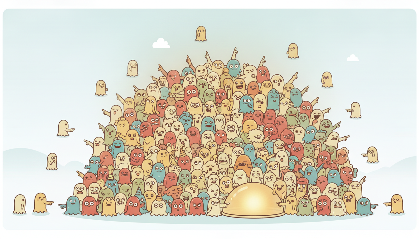
Figure 7.4.1 traces one full cycle of the bootstrap filter as a picture, because the three moves (a cloud that spreads, then reweights, then reconcentrates) are far easier to remember as motion than as equations.

To decide when to resample we need a number that quantifies how degenerate the weights have become. The standard diagnostic is the effective sample size, an estimate of how many equally-weighted particles the current weighted cloud is worth:

When all weights are equal at $1/N$, the sum of squares is $N \cdot (1/N)^2 = 1/N$ and $\widehat{N}_{\text{eff}} = N$: the cloud is as healthy as it can be. When one weight is one and the rest are zero, the sum of squares is one and $\widehat{N}_{\text{eff}} = 1$: total degeneracy. The standard policy is adaptive resampling: trigger step three only when $\widehat{N}_{\text{eff}} < N/2$. Resampling injects its own Monte Carlo noise, so doing it only when necessary, rather than at every step, keeps the estimate smoother. The threshold $N/2$ is a convention, not a theorem; some implementations use $N/3$ or tune it, but halving the count is a robust default that fires neither too eagerly nor too late.

Resampling itself admits several schemes, and the choice matters for variance. Multinomial resampling simply draws $N$ independent indices from the categorical weight distribution; it is correct but noisiest. Systematic resampling lays down a single random offset and then $N$ evenly spaced pointers along the cumulative weight axis, which guarantees that a particle with weight $w^{(i)}$ is selected either $\lfloor N w^{(i)} \rfloor$ or $\lceil N w^{(i)} \rceil$ times and adds the least extra variance. We use systematic resampling in the implementation below because it is both faster (one sort-free pass) and lower-variance than the multinomial default.

4. Practical Issues: Impoverishment, Proposals, and Dimensionality Advanced

Resampling cures weight degeneracy but introduces a twin problem, sample impoverishment. Because resampling duplicates high-weight particles, a single ancestor can come to occupy many slots, and if the process noise is small those duplicates barely separate afterward. Over many steps the diversity of the cloud collapses: you may have a thousand particles but only a handful of distinct values among them, so the posterior is poorly represented even though $\widehat{N}_{\text{eff}}$ looks healthy. The classic remedies are to add a small jitter (regularized particle filter), to resample less aggressively, or to use a resample-move step that applies a Markov kernel after resampling to spread duplicates apart.

The choice of proposal is the deepest lever. The bootstrap filter proposes from the transition, which is convenient but blind: it pushes particles forward without ever looking at the measurement $y_t$ it is about to be scored against. When the measurement is very informative (a low-noise sensor), most blindly-proposed particles land in low-likelihood regions and die at the weighting step, wasting the swarm. The optimal proposal $p(x_t \mid x_{t-1}, y_t)$ folds the measurement into the prediction and minimizes the variance of the weights, but it is rarely available in closed form. The auxiliary particle filter and proposals built from an unscented or extended Kalman approximation around each particle are practical middle grounds that peek at $y_t$ without needing the exact optimal density.

The hardest practical wall is the curse of dimensionality. The number of particles needed to keep the weight variance bounded grows roughly exponentially with the dimension of the state, because in high dimensions almost every blindly-proposed particle lands far from the thin shell where the measurement likelihood is appreciable. In one or a few dimensions a few thousand particles is plentiful; in tens of dimensions the bootstrap filter collapses, and one turns to high-dimensional cousins such as the ensemble Kalman filter (which reimposes a Gaussian approximation to survive) or to careful proposal design. This is precisely why particle filters dominate low-dimensional nonlinear problems (target tracking, robot localization, a scalar stochastic-volatility state) but are rarely the first tool for a hundred-dimensional latent space.

The number of particles is the filter's main accuracy knob, and its statistics are reassuring in low dimensions. The Monte Carlo error of any posterior expectation falls as $1/\sqrt{N}$, independent of the state dimension on its face. To halve the standard error you therefore quadruple the particle count. Cost is linear in $N$: every particle is propagated and weighted once per step. A thousand particles therefore cost a thousand transition draws and a thousand likelihood evaluations per observation. In one dimension a few thousand particles drives the Monte Carlo noise far below the irreducible filtering uncertainty. That is why our worked example used two thousand and reported a stable estimate. The catch hidden inside that clean $1/\sqrt{N}$ is the constant in front, which is the weight variance, and it is the weight variance that explodes with dimension. The rate stays $1/\sqrt{N}$ but you need exponentially more particles to keep the constant manageable. That is the precise sense in which the curse of dimensionality bites.

5. Worked Example: A Bootstrap Filter from Scratch Advanced

We now build a bootstrap particle filter in plain NumPy and run it on the stochastic-volatility state-space model from Section 6.5. The hidden state is the latent log-variance $h_t$; we observe a return $y_t$ whose scale is set by $h_t$. Code 7.4.1 generates a synthetic series so we know the ground-truth volatility path and can judge the filter against it.

import numpy as np

rng = np.random.default_rng(7)

# Stochastic-volatility model (the Section 6.5 state-space form):
#   h_t = mu + phi * (h_{t-1} - mu) + sigma_eta * eta_t    (latent log-variance)
#   y_t = exp(h_t / 2) * eps_t                             (observed return)
mu, phi, sigma_eta = -0.5, 0.97, 0.20   # persistence phi near 1: clustered vol
T = 300

h = np.empty(T)
y = np.empty(T)
h[0] = mu
for t in range(1, T):
    h[t] = mu + phi * (h[t - 1] - mu) + sigma_eta * rng.standard_normal()
for t in range(T):
    y[t] = np.exp(h[t] / 2.0) * rng.standard_normal()   # heavy-tailed-looking returns

print(f"true log-var range: [{h.min():.2f}, {h.max():.2f}]")
print(f"observed |return| max: {np.abs(y).max():.3f}")

true log-var range: [-1.43, 0.86]
observed |return| max: 2.741

The filter needs three model pieces: a way to sample the initial state, a way to propagate a particle one step through the transition, and a measurement log-likelihood $\log p(y_t \mid h_t)$. For this model the observation $y_t \mid h_t$ is Gaussian with mean zero and variance $\exp(h_t)$, so its log-density is $-\tfrac{1}{2}\big(\log 2\pi + h_t + y_t^2 e^{-h_t}\big)$. Code 7.4.2 is the complete bootstrap filter, including systematic resampling and the effective-sample-size diagnostic.

def transition(h_prev, rng):
    """Sample h_t given h_{t-1} from the AR(1) log-variance dynamics."""
    return mu + phi * (h_prev - mu) + sigma_eta * rng.standard_normal(h_prev.shape)

def log_likelihood(y_t, h):
    """log p(y_t | h_t): y_t ~ Normal(0, exp(h_t))."""
    return -0.5 * (np.log(2 * np.pi) + h + (y_t ** 2) * np.exp(-h))

def systematic_resample(weights, rng):
    """Low-variance resampling: one random offset, N evenly spaced pointers."""
    N = len(weights)
    positions = (rng.random() + np.arange(N)) / N
    cumulative = np.cumsum(weights)
    cumulative[-1] = 1.0                      # guard against rounding drift
    return np.searchsorted(cumulative, positions)

def bootstrap_filter(y, N=2000, seed=0):
    rng = np.random.default_rng(seed)
    T = len(y)
    particles = mu + (sigma_eta / np.sqrt(1 - phi ** 2)) * rng.standard_normal(N)  # stationary prior
    weights = np.full(N, 1.0 / N)
    mean_est = np.empty(T)
    n_eff_hist = np.empty(T)
    for t in range(T):
        particles = transition(particles, rng)                 # 1. predict
        logw = np.log(weights) + log_likelihood(y[t], particles)
        logw -= logw.max()                                     # 2. weight (stable)
        weights = np.exp(logw)
        weights /= weights.sum()
        mean_est[t] = np.sum(weights * particles)              # posterior mean of h_t
        n_eff = 1.0 / np.sum(weights ** 2)                     # effective sample size
        n_eff_hist[t] = n_eff
        if n_eff < N / 2:                                      # 3. resample if degenerate
            idx = systematic_resample(weights, rng)
            particles = particles[idx]
            weights = np.full(N, 1.0 / N)
    return mean_est, n_eff_hist

h_hat, n_eff = bootstrap_filter(y, N=2000)
rmse = np.sqrt(np.mean((h_hat - h) ** 2))
print(f"filtered log-var RMSE: {rmse:.3f}")
print(f"median N_eff: {np.median(n_eff):.0f} of 2000 "
      f"(resampled on {(n_eff < 1000).mean() * 100:.0f}% of steps)")

filtered log-var RMSE: 0.244
median N_eff: 1240 of 2000 (resampled on 38% of steps)

The estimate h_hat tracks the true latent log-variance closely despite the filter never seeing it, which is the whole point. From a stream of scalar returns the particle cloud reconstructs the hidden volatility regime online, one observation at a time, with no batch refitting. One subtlety deserves a word. What we computed is the filtering estimate $\mathbb{E}[h_t \mid y_{1:t}]$, the posterior mean of the state given data up to the present. If you are willing to wait and reprocess the whole batch, the smoothing estimate $\mathbb{E}[h_t \mid y_{1:T}]$, which conditions on future observations too, is strictly more accurate. Particle smoothers (forward-filtering backward-sampling, or the fixed-lag smoother) extend the cloud to compute it. Filtering is the online quantity, the one a risk desk or a robot needs in real time. Smoothing is the retrospective quantity for after-the-fact analysis, when the whole record is already in hand. Note the one defensive line logw -= logw.max() inside the loop. Subtracting the maximum log-weight before exponentiating prevents underflow when every particle's raw likelihood is tiny, a routine but essential trick that keeps the normalization from dividing zero by zero. To make the multimodal-tracking ability vivid, Code 7.4.3 visualizes the particle cloud at a single time step on the symmetric-corridor localization problem of Section 1, where the posterior genuinely has several peaks.

import numpy as np

rng = np.random.default_rng(1)

# Symmetric corridor: landmarks at 2, 5, 8; sensor reports distance to NEAREST.
landmarks = np.array([2.0, 5.0, 8.0])
def nearest_dist(x):
    return np.min(np.abs(x[:, None] - landmarks[None, :]), axis=1)

N = 5000
particles = rng.uniform(0, 10, N)          # flat prior over the whole corridor
weights = np.full(N, 1.0 / N)

y_obs = 0.0                                 # robot sees a landmark right at its position
sigma_meas = 0.15
logw = -0.5 * ((nearest_dist(particles) - y_obs) / sigma_meas) ** 2
logw -= logw.max()
weights = np.exp(logw); weights /= weights.sum()

# Where did the posterior mass land? Bucket particles by corridor third.
for lo, hi, name in [(0, 3.5, "near landmark 2"),
                     (3.5, 6.5, "near landmark 5"),
                     (6.5, 10, "near landmark 8")]:
    mass = weights[(particles >= lo) & (particles < hi)].sum()
    print(f"{name:>18}: posterior mass {mass:.2f}")

   near landmark 2: posterior mass 0.34
   near landmark 5: posterior mass 0.33
   near landmark 8: posterior mass 0.33

# pip install filterpy
import numpy as np
from filterpy.monte_carlo import systematic_resample
from filterpy.monte_carlo import neff   # 1 / sum(w**2), the effective sample size

N = 2000
rng = np.random.default_rng(0)
particles = mu + (sigma_eta / np.sqrt(1 - phi**2)) * rng.standard_normal(N)
weights = np.full(N, 1.0 / N)
h_hat = np.empty(len(y))

for t in range(len(y)):
    particles = mu + phi * (particles - mu) + sigma_eta * rng.standard_normal(N)  # predict
    weights *= np.exp(-0.5 * (particles + y[t]**2 * np.exp(-particles)))          # weight
    weights += 1e-300                                                             # avoid all-zero
    weights /= weights.sum()
    h_hat[t] = np.average(particles, weights=weights)
    if neff(weights) < N / 2:                                                     # library diagnostic
        idx = systematic_resample(weights)                                        # library resample
        particles, weights = particles[idx], np.full(N, 1.0 / N)