"Every domain swears its time series is a special snowflake. Then I forecast all of them with the same matrix of past values, and they all complain in exactly the same way."
A Mildly Overfit Forecaster, Confident About Next Tuesday
Temporal data looks wildly different from one field to the next, a tick of stock prices, a ward full of beeping monitors, a decade of river levels, a fleet of vibrating motors, yet underneath the costumes lives one object: a sequence of observations indexed by time, where order carries meaning and the past constrains the future. This section tours seven domains, names what makes each hard, then strips them down to the shared abstraction $x_{1:T}$ that the rest of the book builds on. Master the differences and you choose the right tool; master the commonality and you stop re-learning the same lesson in every new field.
In Section 1.1 we argued that intelligence becomes temporal the moment a system must remember, anticipate, and act under an unfolding flow of information. That was a claim about cognition. This section grounds it in data. Before we can build a forecaster, a filter, or a decision agent, we need to know what temporal data actually looks like in the wild, because the shape of the data, how often it arrives, how noisy it is, how far ahead we must see, dictates almost every modeling choice that follows. A model that thrives on dense audio frames can drown in a sparse stream of clinical labs, and a method tuned for the gentle seasonality of electricity demand can be humiliated by the near-random walk of asset returns. We therefore start concrete, with domains, then ascend to the abstraction that unifies them.
1. A Tour of Seven Domains Beginner
Each domain below is described by four axes that recur throughout the book: its data shape (dimensionality and structure), its sampling regime (how observations are spaced in time), its typical horizon (how far ahead prediction must reach), and its notion of what good prediction means. These axes are not decoration; they map directly onto later chapters, and the comparison in Table 1.2.1 collects them so you can see the contrasts at a glance.
Finance. The canonical series is a stream of asset prices, usually reduced to log returns $r_t = \log(p_t / p_{t-1})$ and their time-varying volatility. Returns are sampled regularly (daily, minutely, or down to microsecond ticks) but are notoriously close to a random walk: tomorrow's return is almost unpredictable in mean, so the signal-to-noise ratio is brutally low and the process is non-stationary, with volatility clustering in calm and turbulent regimes. "Good" prediction here rarely means nailing the next price; it means a small, robust edge in expected return, a calibrated forecast of volatility, or a well-shaped predictive distribution. We return to this series with ARIMA and GARCH in Chapter 5 and with probabilistic deep forecasters in Chapter 19.
Healthcare. A patient generates many vital signs (heart rate, blood pressure, oxygen saturation, lab values) but they are measured whenever a clinician or a device happens to act, so the series is irregularly sampled, multivariate, and riddled with missingness. The very pattern of missingness can be informative: a lab ordered urgently signals concern. Horizons are short and the stakes are absolute, an early-warning model that flags deterioration six hours ahead can save a life, so calibration and a low false-alarm rate matter more than raw accuracy. Irregular clinical data drives the data-engineering of Chapter 2 and the continuous-time neural models of Chapter 13.
Climate and energy. Temperature, wind, river flow, and electricity demand are dominated by strong, nested seasonality (daily, weekly, annual) layered on slow trends, and they obey physical constraints (energy balances, non-negativity, conservation laws). Sampling is regular and horizons stretch long, from day-ahead grid scheduling to multi-decade climate projection. "Good" prediction means respecting the seasonal structure and the physics, and quantifying uncertainty over long lead times. Seasonality and the frequency domain are the subject of Chapter 4.
Industry and IoT. Machines emit sensor telemetry (vibration, temperature, current, pressure) at high, regular rates across many channels. The dominant tasks are not point forecasts but anomaly detection and predictive maintenance: spotting the rare deviation that precedes a failure. Data is plentiful but labels (actual failures) are rare and precious. This is the home of Chapter 8 on anomaly and change-point detection and of the deployment concerns in Chapter 34.
Web and retail. Demand forecasting deals with thousands or millions of related series (every product in every store) that are often intermittent (many zeros between sparse sales) and hierarchical (item rolls up to category rolls up to region, and the levels must reconcile). Sampling is regular but the cross-series structure is the real challenge, and "good" means coherent forecasts across the hierarchy that a planner can act on. Global models that learn across many series, a recurring theme from Chapter 14, were born here.
Audio, speech, and language. Waveforms, spectrogram frames, and token streams are dense, long, and (after framing) regularly spaced sequences. They are the historical bridge from time-series thinking to modern sequence models: the same recurrent and attention machinery that transcribes speech now forecasts demand. These domains motivate the neural sequence fundamentals of Chapter 9 and the attention and Transformer architectures of Chapter 12.
Robotics and control. Here the data is closed-loop: an agent observes a state, takes an action, and that action changes the future observations it will receive. The series is no longer a passive recording but a consequence of decisions, which breaks the assumption that the future is independent of our model's outputs. This closed-loop nature is precisely what Part VI builds on, starting with Markov decision processes in Chapter 22.
| Domain | Sampling | Dimensionality | Noise level | Typical horizon | Dominant task |
|---|---|---|---|---|---|
| Finance | Regular (tick to daily) | Low to moderate | Very high | Short | Return edge, volatility forecast |
| Healthcare | Irregular, event-driven | Moderate, multivariate | High, with missingness | Short (hours) | Early warning, risk scoring |
| Climate and energy | Regular | Low to high (spatial fields) | Low to moderate | Long (days to decades) | Seasonal forecasting |
| Industry and IoT | Regular, high rate | High, many channels | Moderate | Short to medium | Anomaly, predictive maintenance |
| Web and retail | Regular (daily, weekly) | Very high (many series) | Moderate, intermittent | Short to medium | Hierarchical demand forecasting |
| Audio, speech, language | Regular, dense | Moderate to high | Low to moderate | Very short (next frame or token) | Sequence transduction |
| Robotics and control | Regular, closed-loop | Moderate to high | Moderate | Receding (planning horizon) | Sequential decision making |
Reading Table 1.2.1 across the columns reveals the engineering tradeoffs. Finance and healthcare sit at opposite corners of the noise-versus-structure plane; climate and retail both lean on structure (seasonality, hierarchy) that a good model must exploit rather than fight; robotics alone breaks the passive-data assumption that the other six share. Hold these contrasts in mind, because the next subsection asks what survives when we abstract them all away.
The same person can be three domains in one afternoon: a heart-rate trace on a smartwatch (healthcare, irregular when you forget to charge it), the watch's accelerometer stream (IoT, dense and regular), and the spending pattern of the lunch they bought (retail, intermittent and seasonal around paydays). Temporal AI is less a set of separate fields than one habit of mind applied to whatever happens to be ticking.
2. What Every Domain Shares Beginner
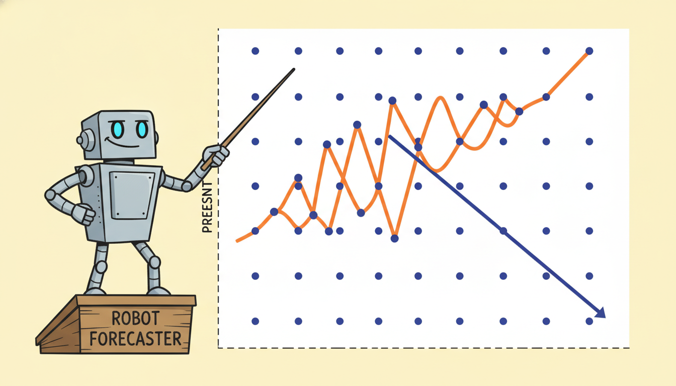
Strip away the vocabulary and the seven domains collapse onto one object. A temporal dataset is a sequence of observations, and the cautionary illustration below shows the trap that waits when a model mistakes past fit for future skill.
where the index $t$ orders the observations in time and $d$ is the number of variables measured at each step (the unified notation of Appendix A uses this $x_{1:T}$ form throughout). Four properties hold across every domain above, and together they are what makes data temporal rather than merely a bag of points.
First, ordering carries information: shuffling the sequence destroys content that a shuffled tabular dataset would not lose, because the relationship between $x_t$ and $x_{t+1}$ is the signal. Second, autocorrelation: nearby observations are statistically dependent, so $x_t$ is partially predictable from its own past, which is exactly what a forecaster exploits and what an anomaly detector treats as the baseline to deviate from. Third, non-stationarity: the data-generating process drifts, the mean wanders, the variance breathes, the seasonal amplitude shifts, so the statistics estimated yesterday may not hold tomorrow, a problem we confront head-on with online learning in Chapter 20. Fourth, and most unifying, the past summarizes into a state: we rarely need the entire history to predict the future; a sufficient summary, a state $s_t$, often captures everything the past says about what comes next.
For regularly sampled data the index is an integer step and the physical times are $t_k = t_0 + k\,\Delta$ for a fixed sampling interval $\Delta$. For irregular data (the clinical case) the observations arrive at arbitrary, strictly increasing timestamps
$$t_1 < t_2 < \dots < t_n,$$and the gaps $\Delta_k = t_k - t_{k-1}$ themselves vary and may carry meaning. The difference between these two regimes, a fixed $\Delta$ versus a sequence of varying $\Delta_k$, is the single most consequential property to check before modeling, and it is exactly what the worked example in Subsection 4 makes tangible.
The idea that the past compresses into a state $s_t$ that is sufficient for the future is the thread that ties this entire book together. The Kalman filter (Chapter 7) makes the state explicit and Gaussian; the recurrent network (Chapter 10) learns the state in a hidden vector; the structured state-space model (Chapter 13) makes that learned state scale to very long sequences; and the belief-state agent of Chapter 23 carries a state under partial observation. Different costumes, one idea: find the summary of the past that the future depends on.
Watch the abstraction $x_{1:T}$ with its state $s_t$ reappear in learned form throughout the book. ARIMA's autoregression (Chapter 5) returns as linear attention (Chapter 13); the hidden Markov model (Chapter 7) returns as the neural latent-variable model (Chapter 17). Recognizing the shared skeleton is what lets one practitioner work across all seven domains of Table 1.2.1.
3. The Three Running Datasets of This Book Beginner
To make the abstraction concrete and to give you a fixed yardstick as methods accumulate, this book carries three running datasets, one regular and noisy, one irregular and multivariate, one regular and high-rate, chosen so that together they exercise the full span of Table 1.2.1. They are introduced here and reappear deliberately in later chapters; the full inventory lives in the table of contents and in Appendix E.
The finance dataset is a daily returns and volatility series derived from an equity index. It is our standing example of a low signal-to-noise, near-random-walk, non-stationary process, and it threads through ARIMA and GARCH (Chapter 5), deep forecasting (Chapter 14), and probabilistic forecasting (Chapter 19).
The healthcare dataset is an irregularly sampled multivariate clinical vitals series with realistic missingness. It is our standing example of event-driven, life-or-death temporal data, and it threads through temporal data engineering (Chapter 2), state-space filtering (Chapter 7), and continuous-time neural models (Chapter 13).
The sensor and IoT dataset is industrial machine telemetry sampled at a high, regular rate across several channels. It is our standing example for anomaly and change-point detection (Chapter 8), drift and online adaptation (Chapter 20), and deployment (Chapter 34).
The point of fixing three datasets is comparability: when a Transformer in Part III and a Kalman filter in Part II are both asked to forecast the same finance series, the difference you observe is a property of the method, not of a changed benchmark. The worked example below builds a small synthetic stand-in for the healthcare and sensor cases so you can run it immediately, before the full datasets are loaded in Chapter 2.
Who: A data science team embedded in the critical-care unit of a regional hospital.
Situation: Nurses already chart vitals, but deterioration on general wards is sometimes caught late, after a patient has begun to crash.
Problem: The team wanted a model that flags patients likely to deteriorate within the next six hours, using only the vitals already being collected.
Dilemma: The data was exactly the healthcare archetype of Table 1.2.1: irregularly sampled, multivariate, heavily missing. They could resample everything onto a fixed hourly grid (simple, but it fabricates values and discards the information in when a measurement was taken), or model the irregular timestamps directly (faithful, but it demands the continuous-time machinery of Chapter 13 and more engineering).
Decision: They started with a carefully resampled hourly grid plus explicit "time since last measurement" and "was this observed" features, so the model could still see the missingness pattern, then planned a continuous-time successor once the baseline proved its worth.
How: Using the resampling and gap-feature techniques previewed in the next subsection and developed fully in Chapter 2, they built an early-warning score recomputed each hour, calibrated so that a fixed alert rate matched the nursing team's capacity to respond.
Result: In a silent trial the score surfaced a meaningful share of deteriorations several hours before the existing manual triggers, at a false-alarm rate the ward could absorb.
Lesson: The sampling regime is not a detail to be smoothed away; the missingness pattern was itself a feature, and the design choice of how to handle irregular timestamps shaped the whole system.
The boldest current bet is that the shared abstraction of Subsection 2 is strong enough to support a single model pretrained across all these domains at once, then applied zero-shot to a series it has never seen. TimesFM (Das et al., Google, 2024) is a decoder-only forecaster trained on a large, heterogeneous corpus; Chronos (Ansari et al., Amazon, 2024) tokenizes scaled time-series values and trains a language-model backbone on them; Moirai (Woo et al., Salesforce, 2024) targets any-variate, any-frequency forecasting; and MOMENT and Lag-Llama pursue the same general-purpose goal. These models lean directly on the premise of this section, that finance, energy, and demand differ in surface statistics but share deep temporal structure, and their early success suggests the unifying view is not just pedagogically convenient but empirically real. We study them in depth in Chapter 15.
4. Worked Example: Regular versus Irregular Sampling in pandas Intermediate
Nothing makes the regular-versus-irregular distinction concrete like building both and resampling them. Code 1.2.1 constructs a small synthetic multivariate series in two flavors: a regularly sampled sensor stream (fixed $\Delta$ of one minute) and an irregularly sampled vitals stream (varying gaps $\Delta_k$), then inspects each.
import numpy as np
import pandas as pd

rng = np.random.default_rng(0)

# --- Regular stream: an IoT sensor sampled every 60 seconds (fixed delta) ---
reg_index = pd.date_range("2026-01-01 00:00", periods=12, freq="1min")
regular = pd.DataFrame(
    {
        "temp_c": 20 + np.cumsum(rng.normal(0, 0.3, 12)),   # drifting temperature
        "vibration": rng.normal(1.0, 0.05, 12),             # near-constant baseline
    },
    index=reg_index,
)

# --- Irregular stream: clinical vitals charted at arbitrary, increasing times ---
offsets_min = np.cumsum(rng.integers(2, 25, size=8))        # varying gaps (minutes)
irr_index = pd.Timestamp("2026-01-01 00:00") + pd.to_timedelta(offsets_min, unit="m")
irregular = pd.DataFrame(
    {
        "heart_rate": rng.normal(78, 6, 8).round(0),
        "spo2": rng.normal(97, 1.2, 8).round(0),
    },
    index=irr_index,
)

print("Regular gaps (s):", np.unique(np.diff(regular.index) / np.timedelta64(1, "s")))
print("Irregular gaps (min):", (np.diff(irregular.index) / np.timedelta64(1, "m")))
print("\nIrregular head:\n", irregular.head(3))
print calls expose the defining contrast: one constant gap versus a sequence of unequal gaps $\Delta_k$.Regular gaps (s): [60.]
Irregular gaps (min): [ 8. 21. 9. 19. 4. 22. 11.]
Irregular head:
heart_rate spo2
2026-01-01 00:08:00 82.0 98.0
2026-01-01 00:29:00 74.0 96.0
2026-01-01 00:38:00 81.0 97.0
The regular stream is trivial to feed into any model that assumes evenly spaced steps. The irregular stream is not, and the standard first move is to resample it onto a fixed grid, which forces a choice about how to fill the gaps. Code 1.2.2 resamples the vitals onto a regular five-minute grid and shows two policies side by side.
# Resample the irregular vitals onto a fixed 5-minute grid.
grid = irregular.resample("5min")

ffill_grid = grid.ffill()                 # carry the last observed value forward
interp_grid = grid.mean().interpolate()   # average within bin, then interpolate gaps

# A "time since last real measurement" feature preserves the missingness signal.
observed = irregular.reindex(ffill_grid.index, method=None).notna()["heart_rate"]
gap_min = (
    ffill_grid.index.to_series()
    - ffill_grid.index.to_series().where(observed).ffill()
).dt.total_seconds() / 60.0

print("Forward-filled grid:\n", ffill_grid["heart_rate"].head(6).to_string())
print("\nMinutes since last real reading:\n", gap_min.head(6).to_string())
Forward-filled grid:
2026-01-01 00:05:00     NaN
2026-01-01 00:10:00    82.0
2026-01-01 00:15:00    82.0
2026-01-01 00:20:00    82.0
2026-01-01 00:25:00    82.0
2026-01-01 00:30:00    74.0

Minutes since last real reading:
2026-01-01 00:05:00    NaN
2026-01-01 00:10:00    2.0
2026-01-01 00:15:00    7.0
2026-01-01 00:20:00    12.0
2026-01-01 00:25:00    17.0
2026-01-01 00:30:00    1.0
If you plot the two series, the regular sensor temperature traces a smooth random-walk drift sampled at evenly spaced points, while the forward-filled heart rate is a staircase: flat plateaus between real readings with abrupt steps where a new measurement lands, a visual reminder that the flat stretches are assumptions, not observations. That staircase is the honest picture of what resampling does, and recognizing it is the first defense against the leakage and fabricated-data pitfalls that Chapter 2 tackles in full.
Hand-rolling resampling, gap features, and per-series alignment for thousands of series is the bulk of a forecasting pipeline. The Nixtla stack collapses it: a single tidy long frame plus one call handles regular gridding, missing-value policies, and even the model fit. The block below forecasts the regular sensor channel in a few lines, with frequency handling, train and predict that would otherwise be dozens of lines of pandas done internally.
# pip install statsforecast
from statsforecast import StatsForecast
from statsforecast.models import AutoARIMA

# Nixtla expects long format: unique_id, ds (timestamp), y (value).
long = (regular.reset_index()
        .rename(columns={"index": "ds", "temp_c": "y"})
        .assign(unique_id="sensor_1")[["unique_id", "ds", "y"]])

sf = StatsForecast(models=[AutoARIMA()], freq="1min")
forecast = sf.forecast(df=long, h=5)      # 5-step-ahead forecast, fitted internally
print(forecast.head())
statsforecast; one forecast call replaces manual gridding, model selection, and the forecast loop, and the identical long-format interface scales to millions of series.Pick a temporal series you have personally generated or care about (your step count, your inbox arrival times, a game's score over a season). Place it on all five axes of Table 1.2.1: sampling regime, dimensionality, noise level, typical horizon, and dominant task. Which of the seven domains does it most resemble, and which axis was hardest to assign? Argue in two sentences what "good prediction" would mean for it.
Extend Code 1.2.2 by resampling the irregular vitals onto three different grids (1-minute, 5-minute, 30-minute) using forward-fill. For each grid, count how many rows are real observations versus fabricated fills, and compute the mean and standard deviation of heart_rate. Explain how and why the summary statistics drift as the grid coarsens, and relate your finding to the "minutes since last real reading" feature: at which grid does that feature stop being informative?
Six of the seven domains in Table 1.2.1 record data passively; robotics and control does not. Write a short analysis of what changes when your model's outputs influence the future data it will see. Give one concrete way a forecasting evaluation that is valid for the finance series would become misleading if naively applied to a control series, and name the chapter (Chapter 22) where the correct framework lives.