"I can remember last Tuesday with perfect clarity and predict next Tuesday with serene confidence. It is the commitment in between, deciding now for a payoff that arrives much later, that keeps me up at night."
A Recurrent Network With Long-Term Commitment Issues
Intelligence is the management of an arrow of time: a system worth calling intelligent takes an ordered stream of past observations, compresses it into a usable summary, turns that summary into predictions about what comes next, and turns predictions into actions whose consequences unfold later. The static classifier that maps one independent input to one label is the degenerate case where the arrow has length zero. Everything in this book lives where the arrow has length: data that arrives in order, models that carry memory, and decisions whose reward is deferred. This section establishes the vocabulary (sequence, horizon, lookback window, latent state) and the single thesis (predict, reason, act) that organizes the other thirty-five chapters.
Most introductory machine learning quietly assumes that the universe hands you a bag of examples in no particular order. You draw a photo, you label it cat or dog, you put it back, you draw another, and the order in which you drew them carries no information. That assumption (the data are independent and identically distributed) is a convenient fiction that makes the mathematics clean and the benchmarks tidy. It is also wrong about almost everything that matters in a deployed system. Prices move in sequence, patients deteriorate over hours, sensors stream telemetry, language arrives word after word, and an agent acting in the world changes the very distribution it will sample next. The moment order carries information, you have left the comfortable land of static prediction and entered temporal intelligence. This section is about what changes, and why that change is the organizing principle of the entire book.
1. Time as the Hidden Axis of Intelligence Beginner
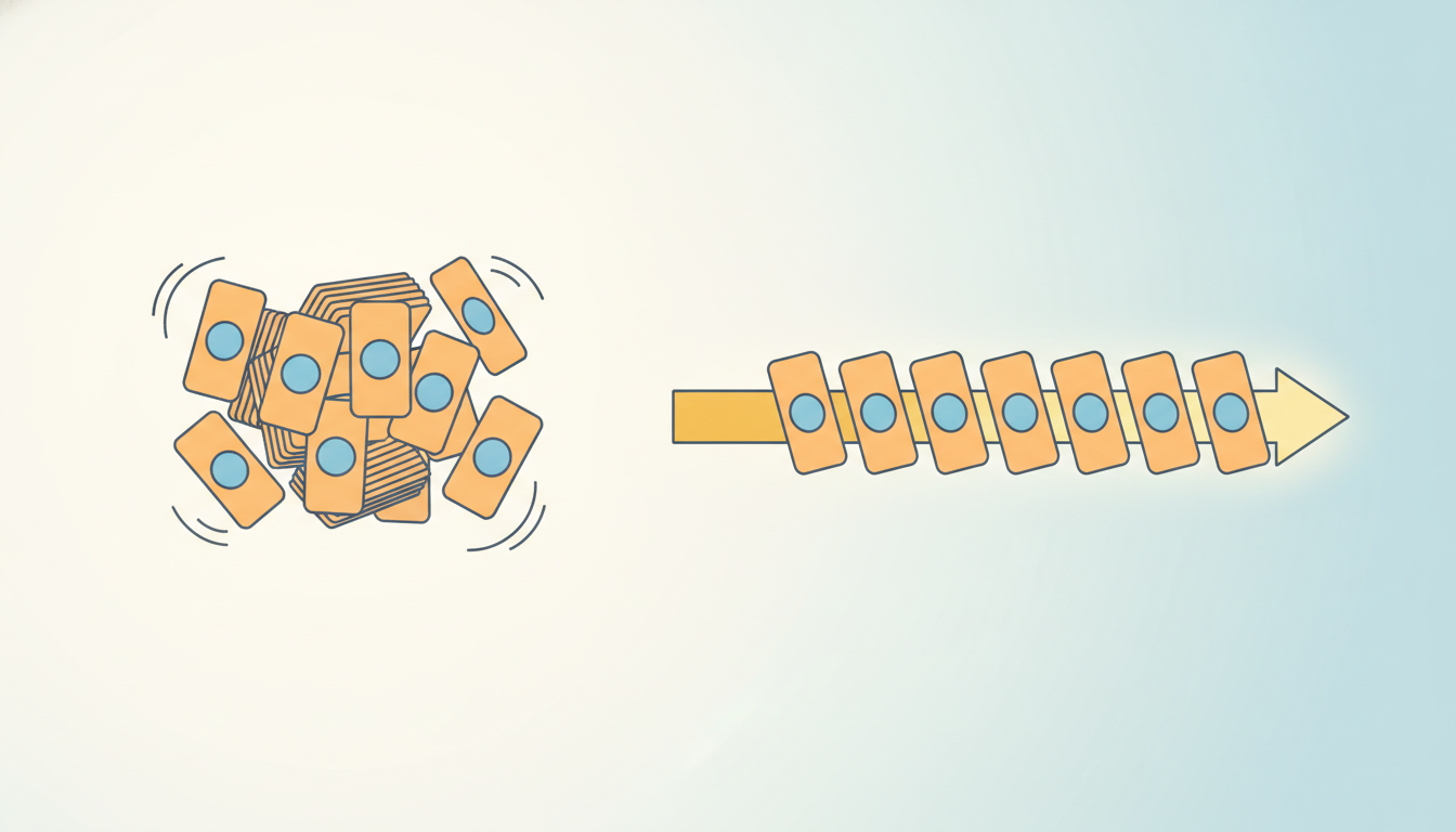
Consider two systems side by side. The first is a static image classifier. It receives a single input $x$, applies a learned function $f$, and emits a label $y = f(x)$. Show it the same image twice and it returns the same answer; permute your test set and its accuracy does not budge. There is no before and no after. The second system is an agent embedded in a stream: a trading model watching a price tick by, a clinical monitor reading vitals, a robot controller closing a loop with the world. At each instant it sees not a fresh independent sample but the next item in an ordered sequence, and its job is to use what came before to anticipate or influence what comes next. The illustration below contrasts these two stances.
We write that stream as a sequence indexed by time. Let $x_t$ denote the observation at step $t$, and write the run of observations from step $1$ up to and including step $t$ as
$$x_{1:t} = (x_1, x_2, \dots, x_t).$$The colon notation $x_{1:t}$ recurs on nearly every page of this book; it is one of the first entries in the unified notation table of Appendix A. The defining feature of a temporal system is that its output at time $t$ is allowed to depend on the whole history $x_{1:t}$, not just on the current $x_t$. Four faculties we casually attribute to intelligence are, on inspection, all operations on that history. Perception integrates a window of recent observations into an estimate of the present state. Memory retains older observations that remain relevant. Anticipation projects the history forward into a guess about $x_{t+1}$ and beyond. Action selects an intervention whose effect will register only in future observations. Strip the time axis away and all four collapse: perception becomes a single snapshot, memory becomes nothing to remember, anticipation becomes nothing to anticipate, and action becomes a one-shot label with no consequence. Time is not one feature among many. It is the axis along which these faculties exist at all.
A static model is a function from input to output. A temporal model is a function from a history to an output, and that single change is the source of every hard problem in this book: histories grow without bound, so the model must compress; the future is only partially determined by the past, so the model must quantify uncertainty; and an acting model perturbs the very stream it is learning from, so training and deployment are no longer the same distribution. The reward for tolerating this difficulty is everything a static model cannot do: forecast, track, plan, and adapt.
2. Why the i.i.d. Assumption Breaks Beginner
The independent-and-identically-distributed assumption underwrites the standard machine learning workflow: shuffle the data, split into train and test, and trust that each example carries the same information regardless of its neighbors. For temporal data this assumption fails in three linked ways. The data are ordered: position carries meaning, and $x_5$ following $x_4$ is a fact about the world, not an accident of storage. The data are autocorrelated: nearby values are statistically dependent, so knowing $x_{t}$ tells you a great deal about $x_{t+1}$. And the data are non-exchangeable: permuting the sequence changes its joint probability, because the joint distribution does not factor into a product of identical marginals. Autocorrelation, informally, is the tendency of a series to resemble time-shifted copies of itself; Chapter 3 makes this precise with the autocorrelation function and the stationarity assumptions that give it meaning.
The cleanest way to feel the difference is to do violence to both kinds of data and measure the damage. Code 1.1.1 builds a tiny autoregressive series (each value a noisy echo of the previous one) and a tiny i.i.d. dataset (independent draws), then shuffles each and asks a simple question: how well does the previous value predict the next one, before and after the shuffle?
import numpy as np

rng = np.random.default_rng(0)
T = 2000

# A temporal series: x_t = 0.9 * x_{t-1} + noise (strong autocorrelation).
x = np.zeros(T)
for t in range(1, T):
    x[t] = 0.9 * x[t - 1] + rng.normal(scale=0.5)

# An i.i.d. "dataset": independent draws, no order information at all.
z = rng.normal(size=T)

def lag1_r2(series):
    """How much of x_t is explained by x_{t-1}? (squared lag-1 correlation)"""
    a, b = series[:-1], series[1:]
    r = np.corrcoef(a, b)[0, 1]
    return r ** 2

print(f"temporal series, in order : lag-1 R^2 = {lag1_r2(x):.3f}")
print(f"temporal series, shuffled : lag-1 R^2 = {lag1_r2(rng.permutation(x)):.3f}")
print(f"i.i.d. data,   in order   : lag-1 R^2 = {lag1_r2(z):.3f}")
print(f"i.i.d. data,   shuffled   : lag-1 R^2 = {lag1_r2(rng.permutation(z)):.3f}")
temporal series, in order : lag-1 R^2 = 0.793
temporal series, shuffled : lag-1 R^2 = 0.001
i.i.d. data,   in order   : lag-1 R^2 = 0.001
i.i.d. data,   shuffled   : lag-1 R^2 = 0.000
This experiment is the cartoon version of a costly real bug. Shuffling an image classification dataset before the train/test split is harmless and recommended; doing the same to a time series silently mixes the future into the training set and inflates your accuracy with information you will not have at deployment. That failure, temporal leakage, is serious enough that Chapter 2 devotes a full section to detecting and preventing it. For now, hold the single takeaway: in temporal data, the ordering is not metadata about the samples, it is the signal.
The phrase "past performance is no guarantee of future results", required on financial products, is a legally mandated confession that the i.i.d. assumption is broken. If returns were truly independent across time, past performance would be a perfectly fair sample of future performance and the disclaimer would be unnecessary. The warning exists precisely because the data are non-stationary: the distribution that generated yesterday is not the distribution that will generate tomorrow. Half of this book is, in a sense, an extended response to that disclaimer.
3. The Three Temporal Verbs: Predict, Reason, Act Intermediate
Once order carries information, three distinct things become worth doing with it, and they form the thesis of this book. The first verb is predict: extrapolate the future from the past. Given the history $x_{1:t}$, produce a guess about what comes next. The canonical target is the one-step-ahead conditional expectation,
$$\hat{x}_{t+1} = \mathbb{E}\!\left[x_{t+1} \mid x_{1:t}\right],$$the value that minimizes expected squared error given everything observed so far. More generally a forecaster predicts an entire stretch $x_{t+1:t+h}$ over a horizon $h$, and an honest one returns not a point but a distribution $p(x_{t+1:t+h} \mid x_{1:t})$, because the future is uncertain and a forecast without uncertainty is a guess wearing a lab coat. Prediction is the subject of Parts II and III, from classical ARIMA and state-space models through recurrent, convolutional, and Transformer forecasters.
The second verb is reason: infer the hidden causes and temporal relations behind the stream. Observations are usually shadows of latent structure (a market regime, a patient's underlying physiological state, a machine's wear level) that we never see directly but must deduce from the sequence. Reasoning also means recovering temporal relations: what preceded what, what caused what, what would have happened under a different intervention. This is the work of Part IV (learning temporal representations and latent-variable models) and Part VII (temporal reasoning and causality). The third verb is act: choose interventions whose payoff unfolds over time. An acting system does not merely observe the stream; it perturbs it, and must trade an immediate cost against a deferred and uncertain reward. That is the defining difficulty of sequential decision making, the subject of Part VI, from Markov decision processes through deep reinforcement learning and planning.
These three verbs are the spine of Building Temporal AI, and the nine parts are their elaboration. Predict runs through Parts II and III (classical forecasting and temporal deep learning) and Part V (uncertainty and online adaptation). Reason runs through Part IV (temporal representation learning) and Part VII (reasoning and causality). Act runs through Part VI (sequential decision making). The same arrow of time underlies all three: prediction turns the past into expectations, reasoning turns observations into latent understanding, and action turns understanding into interventions. Whenever a later chapter feels like a new topic, ask which of the three verbs it serves; it will be one of them. The full map of how chapters realize this thesis lives in the table of contents.
4. Memory and Horizon: How Far Back, How Far Forward Intermediate
Every temporal model, however it is built, makes two commitments that determine its character. The first is how far back it looks: the lookback window (also called the context length or receptive field) is the span of past observations the model is allowed to condition on. The second is how far forward it commits: the horizon $h$ is the number of future steps it must predict or the depth over which its actions accrue consequences. A model with a one-step lookback and a one-step horizon is myopic in both directions; a model that conditions on the full history and plans many steps ahead is ambitious in both, and pays for it in memory, compute, and the difficulty of training. The illustration below pictures these two dials as one figure looking back and ahead.
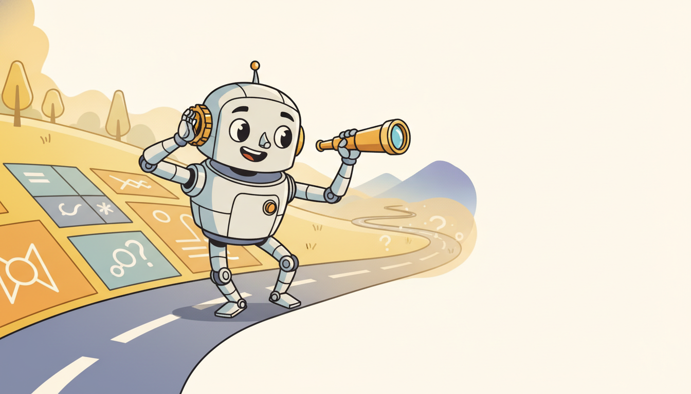
These two quantities are in tension, and the tension is the recurring drama of temporal modeling. Remembering more of the past costs storage and makes the relevant signal harder to find amid the irrelevant; the longer the lookback, the more a model must learn to forget. Committing further into the future compounds uncertainty, because errors accumulate: a forecaster that is slightly wrong at step $t+1$ feeds that error into its guess for $t+2$, and the cloud of plausible futures widens with every step of the horizon. This is the kernel of truth in our chapter's epigraph. A recurrent network really does remember the recent past with ease and predict the near future with confidence; what genuinely strains it is the long-range commitment, holding a fact across hundreds of steps, or choosing an action now whose reward will not arrive for a long time. That difficulty has a name in the recurrent setting (the vanishing-gradient problem) and motivates much of Chapter 10; it has an analogue in decision making (the long-horizon credit-assignment problem) that drives much of Part VI.
Almost every modeling choice in this book can be read as a position on two dials: how much past to condition on (lookback) and how far ahead to commit (horizon). A moving average sets a short lookback; an attention layer sets a long, content-addressed one. A one-step forecaster sets $h = 1$; a planner sets $h$ to the depth of its rollouts. When you meet a new architecture, locate it on these two dials first, and much of its behavior, its cost, its strengths, and its failure modes will follow.
5. A First Taste of the Unifying View: Latent State Advanced
The history $x_{1:t}$ grows without bound, yet no practical model can carry an ever-lengthening list of every observation it has ever seen. The resolution to this, and the single most important idea in the book, is the latent state: a fixed-size summary $h_t$ of the past that is sufficient for the future. Formally, $h_t$ is a good state if conditioning on it makes the future independent of the older history,
$$p\!\left(x_{t+1} \mid h_t\right) \approx p\!\left(x_{t+1} \mid x_{1:t}\right),$$so that everything the unbounded past has to say about what comes next is already squeezed into the bounded vector $h_t$. The whole game of temporal modeling is to design or learn an update rule that maintains such a summary, folding each new observation $x_t$ into the running state, $h_t = g(h_{t-1}, x_t)$, and reading predictions out of it. Compress the past into a state, advance the state, predict from the state: that is the loop, and almost every model you will meet is a particular choice of what the state is and how it updates.
The latent-state loop is the deepest of the temporal threads in this book, and you will meet the same idea wearing three costumes. In the Kalman filter (Chapter 7) the state is a Gaussian belief and the update is exact linear-algebraic inference, optimal for linear systems. In the recurrent neural network (Chapter 10) the state is a learned hidden vector and the update $g$ is a trained nonlinear function, trading optimality for the ability to model arbitrary dynamics. In the structured state-space model (Chapter 13) the two are reconciled: a linear recurrence chosen so that it can be unrolled as a long convolution, giving Kalman-like structure with neural-network scale. Three chapters, three mechanisms, one principle: a compressed summary of the past, sufficient for the future. The complete set of these classical-to-neural arcs is catalogued in the cross-reference map that accompanies the contents.
Holding this unifying view changes how the rest of the book reads. Forecasting, filtering, representation learning, and even decision making (where the latent state becomes the agent's belief about a hidden world, the subject of Chapter 23) are all variations on maintaining a sufficient summary of the past and acting on it. With that thread in hand, the next section turns from the abstract question of what makes intelligence temporal to a concrete tour of where temporal data actually comes from.
The lesson of Code 1.1.1, never shuffle before splitting, is easy to state and easy to forget under deadline. Rather than hand-rolling index arithmetic for a leakage-free split, scikit-learn ships a splitter that respects order and even rolls the boundary forward for cross-validation, replacing a dozen error-prone lines:
# Order-preserving cross-validation: every training fold lies strictly
# before its test fold, so no future ever leaks into the past.
import numpy as np
from sklearn.model_selection import TimeSeriesSplit

series = np.arange(12)            # stand-in for x_{1:T}, already in time order
for train_idx, test_idx in TimeSeriesSplit(n_splits=3).split(series):
    print("train:", train_idx, " test:", test_idx)
TimeSeriesSplit from scikit-learn produces forward-chaining folds (train always precedes test), enforcing the no-shuffle rule of Code 1.1.1 automatically. It handles the index bookkeeping that a hand-written split gets subtly wrong, the kind of bug that Chapter 2 dissects in full.Who: A data scientist on the demand-planning team of a regional grocery chain, asked to forecast next-week sales per store so the supply team could pre-position inventory.
Situation: Three years of daily per-store sales were available. The team's standard tabular pipeline, inherited from a fraud-detection project, shuffled all rows and held out a random 20% as a validation set before fitting a gradient-boosted model on lagged features.
Problem: The model reported a stunning validation accuracy, a mean absolute percentage error near 4%, and was promoted to production on that number. In the first live week, error ballooned past 20%, and the supply team over-ordered perishables across forty stores.
Dilemma: Three explanations competed. Perhaps the live week was simply anomalous and the model was fine. Perhaps the features were too weak and the model needed more signal. Or perhaps the evaluation itself was dishonest, the validation number measuring something the model would never get to do in production.
Decision: Rather than add features or blame the week, the scientist re-ran the exact diagnostic of Code 1.1.1 on the pipeline: shuffle the data, and the apparent accuracy survives; respect time order, and it collapses. That collapse is the signature of leakage.
How: They replaced the random split with a forward-chaining TimeSeriesSplit (Code 1.1.2), so every validation fold lay strictly after its training fold, then refit and re-measured. The honest validation error came back near 18%, matching the live week almost exactly.
Result: The 4% number had been pure fiction: with shuffling, each store's neighboring days (which look almost identical) sat on both sides of the split, so the model was effectively interpolating between known points rather than extrapolating into an unknown future. The corrected pipeline forecast worse on paper but honestly, and the over-ordering stopped.
Lesson: The most expensive bug in temporal machine learning is not a weak model; it is an evaluation that quietly assumes i.i.d. data. Order is the signal, and a split that ignores order measures a task the model will never actually face.
The latent-state view and the predict/reason/act thesis are not period pieces; they organize the field's current frontier. The most visible recent shift is the arrival of time-series foundation models, large sequence models pretrained on enormous and diverse collections of series, then applied to new series with little or no task-specific training. Amazon's Chronos (2024) tokenizes numeric values and reuses a language-model backbone; Google's TimesFM (2024) is a decoder-only forecaster pretrained on billions of time points; Salesforce's Moirai (2024) targets any-variate, any-frequency universal forecasting; Lag-Llama and MOMENT (2024) pursue open foundation models for forecasting and general temporal tasks. The headline capability is in-context forecasting, also called zero-shot forecasting: the model conditions on a never-before-seen history and extrapolates without any gradient update, the lookback window of Section 4 doing the work that training once did. A parallel frontier under the act verb is the use of large sequence models as decision makers (the Decision Transformer lineage and modern world-model planners such as Dreamer V3), treating control as conditional sequence prediction. Every one of these systems is, underneath, a particular answer to this section's questions: what is the state, how far back does it look, and how far forward does it dare to commit.
For each of the following, decide whether the data are genuinely temporal (order carries information) or effectively i.i.d., and justify your answer in one or two sentences: (a) the daily closing price of a stock; (b) a folder of independent passport photographs to be classified by country; (c) the sequence of moves in a single chess game; (d) hourly readings from a vibration sensor on a pump; (e) a survey in which 5000 unrelated people each rate one movie once. For the temporal cases, name the lookback window and horizon you would choose for a one-day-ahead or one-move-ahead task, and explain which of the three verbs (predict, reason, act) the task primarily exercises.
Extend Code 1.1.1. Generate the same autoregressive series, then fit a one-step-ahead linear predictor ($\hat{x}_{t+1} = a\,x_t + b$) two ways: once with a forward-chaining split (train on the first 80% of time steps, test on the last 20%) and once with a random shuffled 80/20 split. Report the test mean squared error under each protocol. Then sweep the autoregressive coefficient from $0.0$ to $0.95$ and plot the gap between the two test errors against the coefficient. At what level of autocorrelation does shuffling begin to materially misstate performance, and why does the gap vanish as the coefficient approaches zero?
Pick three temporal systems you have used or read about (for example a spell-checker's next-word suggestion, a thermostat, and a music-recommendation feed). For each, describe in prose what its latent state $h_t$ plausibly summarizes, how that state is updated as new observations arrive, and roughly how long a fact must persist in the state to be useful (its effective lookback). Then argue which of the three mechanisms previewed in Section 5 (a Kalman-style belief, a learned recurrent vector, or a structured state-space recurrence) is the most natural fit for each system, and what would go wrong if you chose one of the others.