"For twenty thousand revolutions a minute I sang the same clean note. Then, three weeks before anyone noticed, a single ball in my outer race began to whisper a frequency that was not in the score: once per shaft turn, then a little harmonic, then a little more. I tried to tell them in the language I had, a faint sideband nobody reads. By the time the floor heard me with their own ears, I had already written my own obituary in the spectrum."
A Vibration Sensor That Heard the Bearing Fail Three Weeks in Advance
A spinning machine broadcasts its health continuously, in the high-frequency texture of its vibration, the slow creep of its temperature, the ripple of its motor current. Predictive maintenance is the discipline of listening to those streams and acting before failure, and it turns out to be not one problem but three coupled temporal problems stacked on top of each other. First, detection: is this machine still behaving normally, or has a fault signature appeared, the anomaly and change-point question of Chapter 8 applied to a sensor tape. Second, prognosis: given that degradation has started, how much useful life remains, a remaining-useful-life (RUL) regression that is the maintenance cousin of the time-to-event modeling of Chapter 18. Third, decision: when do we actually stop the line and replace the part, a sequential decision under uncertainty whose cost structure (a false alarm wastes a good part and a shift of downtime; a missed failure destroys the machine and possibly the operator) is the safe-RL and decision-aware-evaluation territory of Part VI and Chapter 19. This section threads the book's sensor/IoT running dataset through all three, building a complete run-to-failure pipeline, spectral fault features, a degradation/anomaly score, an RUL estimate with a prognostic horizon, from scratch and then in a handful of library lines. It is where the spectral analysis of Chapter 4, the anomaly detection of Chapter 8, the self-supervision of Chapter 16, the drift handling of Chapter 20, and the edge constraints of Chapter 34 stop being separate chapters and become one deployed system.
The sensor/IoT thread has run quietly through this book. In Chapter 8 we detected anomalies and change-points in machine telemetry; in Chapter 20 we watched that telemetry drift as operating conditions shifted; in Chapter 32 we modeled a whole factory floor of correlated sensors spatio-temporally; in Chapter 34 we worried about running the resulting model on a microcontroller bolted to the machine. This section is the payoff. Predictive maintenance is the canonical industrial use of temporal AI, the place where "predict the future of a time series and act on it" has a dollar value attached to every decision, and it exercises almost every technique the book has built. We will be explicit about which earlier idea each pipeline stage reuses, because the engineering reality is that a maintenance system is an assembly of book chapters, not a single model.
The competencies this section installs are four. To frame a maintenance problem as the three coupled temporal tasks (detection, prognosis, decision) and know which book chapter supplies each. To extract physically meaningful fault features from a vibration stream using the envelope-spectrum machinery of Chapter 4, and to weigh those hand-features against learned representations. To build a run-to-failure pipeline end to end: spectral features, a degradation score, and an RUL estimate with a stated prognostic horizon. And to reason about the operational realities, extreme class imbalance, label scarcity, cross-machine drift, edge limits, and the asymmetric cost of false alarms versus missed failures, that decide whether a maintenance model is deployable or merely accurate on paper.
1. The Setting: Three Tasks Hiding in One Sensor Stream Beginner
A modern machine, a pump, a gearbox, a CNC spindle, a wind-turbine drivetrain, carries instrumentation that produces several simultaneous high-frequency streams. An accelerometer on the bearing housing samples vibration at tens of kilohertz; a thermocouple reports temperature at a few hertz; a current clamp on the motor reports the electrical signature at line frequency and its harmonics. Together these form a multivariate sensor tape $\mathbf{x}_{1:T}$ exactly like the running sensor/IoT series of this book, except that here the tape ends, sooner or later, in a failure. The defining data structure of predictive maintenance is the run-to-failure trajectory: a sequence that starts with a healthy machine and runs until the component breaks, so the label we ultimately care about, time remaining until failure, is read off the end of the sequence rather than annotated by a human.
What makes maintenance a rich temporal problem rather than a single forecast is that one sensor stream supports three distinct tasks, each drawing on a different part of this book, and a real system runs all three.
- Fault detection asks a binary, online question: has the machine departed from its healthy operating distribution? This is the anomaly and change-point detection of Chapter 8, applied to streaming telemetry. The detector fires when a fault signature first appears, marking the transition from healthy to degrading.
- Remaining-useful-life prognosis asks a continuous, forward question: given that degradation has begun, how many cycles or hours of useful life remain? This is a regression onto a time-to-event target, the maintenance form of the event and survival modeling of Chapter 18.4, where instead of a hazard over discrete events we estimate a scalar RUL with an uncertainty band.
- Maintenance scheduling asks a sequential-decision question: given the detector's alarm and the prognosis's estimate, when do we actually intervene? Each day we choose to keep running (cheap if the machine survives, catastrophic if it fails) or to stop and service (a guaranteed but bounded cost). That is a sequential decision under uncertainty with an explicit cost structure, the safe-reinforcement-learning and control territory of Part VI.
The three tasks form a pipeline in time. Detection flips first and starts the prognostic clock; prognosis estimates how long the clock has left; the decision policy reads both and picks the moment to act. Crucially they are coupled, not independent: a good RUL estimate makes the decision easy (act when estimated life drops below the lead time you need to schedule a repair), and a reliable detector keeps the prognosis from being asked to extrapolate on a machine that is still perfectly healthy. Figure 35.3.1 lays out the three-stage flow and names the book chapter behind each stage.
The temptation, especially after a book full of powerful sequence models, is to imagine predictive maintenance as one big network that eats raw sensor data and emits a "replace now" signal. Real deployed systems almost never look like that, and not because the network could not in principle learn it. They are a stack: a signal-processing front end that turns vibration into physically interpretable features (Chapter 4), a detector that flags the onset of abnormality (Chapter 8), a prognostic regressor that estimates remaining life (Chapter 18), and a decision policy that converts the estimate into an action under an asymmetric cost (Part VI). The value of the stack is that each layer is separately testable, separately interpretable, and separately replaceable, properties a monolithic black box trained on a handful of failures cannot offer. The book's chapters are, almost exactly, the layers of a maintenance system.
2. The Signal-Processing Backbone: Reading Faults in the Spectrum Intermediate
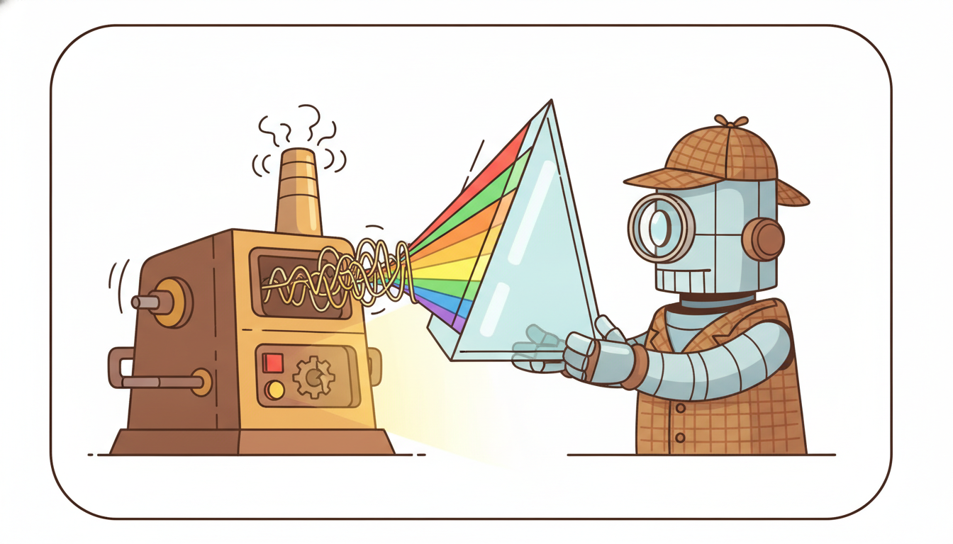
The single most important fact about machine vibration is that faults announce themselves at predictable frequencies. A rolling-element bearing has a geometry, a number of balls, a pitch diameter, a contact angle, and a defect on its outer race strikes the rolling elements at a characteristic rate, the ball-pass frequency of the outer race (BPFO), every time a ball rolls over the flaw. A gear mesh rings at the tooth-pass frequency; a misaligned shaft shows energy at once and twice the rotation rate; an unbalanced rotor concentrates energy at exactly the shaft speed. These are not learned patterns; they are consequences of physics and geometry, and they are the reason the frequency-domain machinery of Chapter 4 is the natural language of fault detection. A healthy machine has a clean spectrum dominated by the running speed and its harmonics; a fault injects energy at its own signature frequency and the sidebands around it.
There is a subtlety that makes raw spectral analysis insufficient and motivates the technique practitioners actually use. A bearing defect produces a series of short, sharp impacts, and those impacts excite a high-frequency structural resonance of the housing. The defect's own repetition rate (a few hundred hertz) is buried under that ringing resonance (several kilohertz) and is hard to see directly in the raw spectrum. The fix is envelope analysis: band-pass the signal around the resonance, take the amplitude envelope (the magnitude of the analytic signal, via the Hilbert transform), and compute the spectrum of that envelope. The envelope spectrum strips away the carrier resonance and reveals the slow repetition rate of the impacts, BPFO, BPFI, and their harmonics, as clean peaks. Envelope analysis is the workhorse of bearing diagnostics, and it is a direct application of the analytic-signal and spectral tools of Chapter 4.
From the envelope spectrum and the raw waveform we extract a compact feature vector that summarizes machine health. The classic hand-features are a mix of time-domain statistics and frequency-domain peaks:
$$\text{RMS} = \sqrt{\tfrac{1}{N}\textstyle\sum_i x_i^2}, \qquad \text{Kurtosis} = \frac{\tfrac{1}{N}\sum_i (x_i - \bar{x})^4}{\big(\tfrac{1}{N}\sum_i (x_i - \bar{x})^2\big)^2}, \qquad \text{CrestFactor} = \frac{\max_i |x_i|}{\text{RMS}}.$$RMS tracks overall energy and rises slowly as a fault grows; kurtosis and crest factor are sensitive to the impulsiveness a fresh defect introduces (a sharp spike on an otherwise smooth wave drives both up) and are early indicators before RMS has moved much; and the amplitude at BPFO in the envelope spectrum is the direct, physically interpretable fault indicator. These features are the input to the detector and the prognostic regressor in the worked pipeline of subsection five.
The whole of Part III taught networks that learn their own features from raw sequences, and Chapter 16 taught them to do so self-supervised, without labels. So why hand-craft RMS, kurtosis, and BPFO amplitude at all? Because in maintenance the number of failures you have ever observed is tiny (often single digits per fault mode), and a feature you derived from bearing physics carries information a network cannot extract from three example failures. The honest trade is this: when failures are abundant (a large fleet, many run-to-failure curves), learned representations win and you should let the network discover the signatures; when failures are scarce, physics-based features are a powerful prior that prevents the model from overfitting noise. The strongest production systems are hybrid, feeding hand features and a learned embedding into the same head, so the physics anchors the model where data is thin and the learning adds nuance where data is thick.
There is something almost literary about envelope analysis. A bearing with an incipient outer-race defect cannot speak, but every time a ball rolls over the flaw it taps out a pulse at exactly BPFO, like a prisoner tapping code on a pipe. The raw vibration drowns that code in the ringing of the housing, the equivalent of shouting over the tapping. Envelope analysis is the act of pressing your ear to the pipe and filtering out the shout: demodulate the carrier, and the patient periodic tapping emerges, spelling out the defect's name in the spectrum. The machine has been confessing the whole time; we just needed the right filter to read the confession.
3. Operational Realities: Why Accurate Models Fail in the Field Advanced
A maintenance model that scores well on a held-out test set routinely fails on a real factory floor, and the reasons are not modeling subtleties but four blunt operational facts. Each maps to a chapter of this book, and ignoring any one of them is the usual cause of a pilot that never reaches production.
Extreme class imbalance. Machines spend almost all of their life healthy. A year of one-second telemetry is 31 million samples; the failure window might be a few hours. The positive class (imminent failure) can be one part in $10^4$ or rarer, so a classifier that always predicts "healthy" achieves better than 99.99 percent accuracy and is completely useless. This is why detection is framed as anomaly detection (Chapter 8): you model the healthy distribution and flag departures from it, rather than training a balanced classifier on a class you have barely seen. Evaluation must use precision, recall, and the cost-weighted metrics of subsection four, never raw accuracy.
Label scarcity. Run-to-failure curves are expensive: each one is a destroyed machine. A fleet might yield dozens of complete failure trajectories, not the millions of labeled examples deep learning expects. This is the natural home of the self-supervised representation learning of Chapter 16: pre-train an encoder on the abundant unlabeled healthy telemetry (predicting masked segments, contrasting augmentations), then fine-tune a small prognostic head on the few labeled failures. The self-supervised pre-training turns the ocean of healthy data, otherwise useless for a supervised RUL model, into a representation that makes the scarce labels go much further.
Drift across machines and conditions. Two nominally identical pumps have different baseline vibration because of installation, foundation stiffness, and wear history; the same pump's signature shifts with load, ambient temperature, and product being processed. A model trained on machine A and deployed on machine B, or trained in summer and run in winter, faces exactly the concept and covariate drift of Chapter 20. Maintenance systems handle this with per-machine baseline normalization (referencing each machine's own healthy fingerprint), operating-condition conditioning, and online adaptation that updates the healthy model as conditions evolve without forgetting what a fault looks like.
Edge deployment constraints. The sensor is bolted to a machine that may be in a mine, on a turbine nacelle, or down a well, with intermittent connectivity and a power budget measured in milliwatts. High-frequency vibration cannot be streamed to the cloud raw (the bandwidth is prohibitive), so feature extraction and often the detector itself must run on a microcontroller at the edge, the quantization, pruning, and latency concerns of Chapter 34. The architecture this forces, extract compact features at the edge, send only those upstream, run heavy prognosis in the cloud, is the standard industrial-IoT topology and a direct consequence of the deployment chapter's constraints.
Who: A reliability-engineering team at an operator of a 60-turbine offshore wind farm, instrumenting each gearbox with accelerometers and streaming the sensor/IoT telemetry threaded through Chapter 32 and this section.
Situation: Gearbox replacement at sea requires a jack-up vessel booked weeks ahead and costs on the order of a quarter-million dollars per event, so an unplanned failure is far more expensive than a scheduled one; a prognostic horizon of three to four weeks was the operational requirement, enough lead time to book the vessel.
Problem: Their first model, a supervised RUL regressor trained on the seven historical gearbox failures in the fleet, scored beautifully offline but raised constant false alarms in service, because winter load patterns shifted every gearbox's baseline vibration and the model read the shift as incipient failure.
Dilemma: Retrain continuously and risk the model adapting to a slow real fault (forgetting what failure looks like); freeze the model and accept the seasonal false alarms; or restructure so the baseline drift was handled separately from the fault signal.
Decision: They split the problem along the book's chapter lines. A self-supervised encoder (Chapter 16) pre-trained on years of unlabeled healthy telemetry gave a representation robust to load; per-turbine baseline normalization (Chapter 20) referenced each gearbox to its own healthy fingerprint, conditioned on load bin, so seasonal shifts canceled; the BPFO envelope feature (Chapter 4) provided a drift-immune physical fault indicator; and the detection threshold was set by the cost analysis of subsection four rather than a default.
How: Edge nodes on each nacelle computed envelope features (Chapter 34) and streamed only the compact vectors ashore, where the prognostic head ran and emitted an RUL with an uncertainty band; an alarm fired only when the lower band crossed the four-week horizon.
Result: False alarms fell by roughly an order of magnitude across the following winter while the detector still caught a genuine outer-race spall with about a 25-day lead, comfortably inside the vessel-booking window, and the gearbox was changed on a planned outage.
Lesson: The accuracy of the RUL model was never the bottleneck; drift, baseline normalization, and the cost-calibrated threshold were. A maintenance system lives or dies on the operational realities of this subsection, not on the prognostic architecture.
4. The Cost Trade-off: False Alarms versus Missed Failures Advanced
Every maintenance decision is a bet under an asymmetric cost, and getting the asymmetry right matters more than getting the model marginally more accurate. There are two ways to be wrong, and they cost wildly different amounts. A false alarm (predict failure, machine was fine) wastes a healthy part and a window of downtime: a real but bounded cost, call it $C_{\text{FA}}$. A missed failure (predict healthy, machine breaks) incurs the full cost of an unplanned catastrophic failure: secondary damage to the machine, an emergency repair, lost production, possibly a safety incident, call it $C_{\text{MF}}$, typically ten to a hundred times larger than $C_{\text{FA}}$. This is the decision-aware evaluation theme of Chapter 19.6: the metric that matters is not detection accuracy but expected cost, and the optimal operating point is set by the cost ratio, not by a default threshold of one half.
The detector emits a score $s$ (an anomaly score or a calibrated failure probability $p$), and we choose a threshold $\tau$ above which we act. The expected cost of acting versus not acting, given failure probability $p$, makes the optimal decision rule explicit. Act (do maintenance) when the expected cost of acting is below the expected cost of waiting:
$$\underbrace{C_{\text{FA}}(1-p)}_{\text{act, but it was fine}} \;<\; \underbrace{C_{\text{MF}}\,p}_{\text{wait, and it fails} } \quad\Longleftrightarrow\quad p \;>\; \frac{C_{\text{FA}}}{C_{\text{FA}} + C_{\text{MF}}} \;\equiv\; \tau^{\star}.$$The optimal threshold $\tau^{\star}$ depends only on the cost ratio. When a missed failure costs 50 times a false alarm, $\tau^{\star} = 1/51 \approx 0.02$: you act on a mere two percent failure probability, accepting many false alarms to avoid the rare ruinous miss. This single formula is why maintenance thresholds are set so low and why raw accuracy is the wrong metric: at $\tau^\star = 0.02$ the system deliberately trades precision for recall because the cost structure demands it. The full sequential version, where each day you also weigh the option of waiting one more day for more information, is the stopping-time and safe-RL problem of Part VI; the static threshold above is its myopic one-step approximation and is what most deployed systems use.
A bearing replacement on a planned outage (the false-alarm cost) is about \$2{,}000 in part plus a scheduled-downtime slot. An unplanned seizure (the missed-failure cost) destroys the shaft and housing, triggers an emergency call-out, and idles the line: estimate \$100{,}000. The cost ratio is $C_{\text{MF}}/C_{\text{FA}} = 50$, so the optimal threshold is $\tau^{\star} = C_{\text{FA}}/(C_{\text{FA}}+C_{\text{MF}}) = 2000/102000 \approx 0.0196$, about two percent. Now compare two operating points on the detector's curve. Point A (threshold tuned for accuracy) catches 70 percent of failures with 1 false alarm per 100 healthy machine-months; point B (threshold at $\tau^\star$) catches 98 percent of failures with 8 false alarms per 100 machine-months. Over a fleet running 100 machine-months with a 3 percent failure rate (3 failures expected), point A misses about 0.9 failures (cost $0.9 \times 100{,}000 = \$90{,}000$) and raises 1 false alarm ($\$2{,}000$), total \$92{,}000. Point B misses about 0.06 failures (cost \$6{,}000) and raises 8 false alarms ($\$16{,}000$), total \$22{,}000. The low, cost-calibrated threshold is four times cheaper despite eight times the false alarms, because the asymmetry makes a missed failure the dominant term. Accuracy would have chosen point A and lost.
5. Worked Example: A Run-to-Failure Pipeline End to End Advanced
We now build the complete pipeline on synthetic run-to-failure data that mimics a degrading bearing: a healthy phase with clean vibration, then a defect that grows, injecting impulsive energy at BPFO and lifting RMS and kurtosis, until failure. The plan follows Figure 35.3.1 exactly. Code 35.3.1 generates the run-to-failure signal and extracts the spectral and statistical health features of subsection two from scratch. Code 35.3.2 builds a degradation/anomaly score and fits a linear RUL estimate with a prognostic horizon. Code 35.3.3 replaces the hand-built pipeline with a few library lines and states the line-count reduction. The point is to make every concept in subsections one through four executable on one trajectory.
import numpy as np

rng = np.random.default_rng(7)
fs = 12000                      # accelerometer sample rate, 12 kHz
shaft_hz = 30.0                 # 1800 rpm shaft speed
bpfo_hz = 3.585 * shaft_hz      # outer-race ball-pass freq, ~3.585x shaft for a typical 9-ball deep-groove bearing
n_cycles = 200                  # 200 run-to-failure measurement cycles (one fault grows)
win = 4096                      # samples per cycle snapshot

def make_cycle(severity):
    """One vibration snapshot. 'severity' in [0,1] is hidden fault growth."""
    t = np.arange(win) / fs
    base = 0.5 * np.sin(2*np.pi*shaft_hz*t)          # healthy: shaft rotation tone
    noise = 0.1 * rng.standard_normal(win)
    # fault: periodic BPFO impacts, amplitude growing with severity, exciting a 3 kHz resonance
    impacts = np.zeros(win)
    period = int(fs / bpfo_hz)
    ring = np.exp(-np.arange(120) / 25.0) * np.sin(2*np.pi*3000*np.arange(120)/fs)
    for k in range(0, win - 120, period):
        impacts[k:k+120] += severity * ring
    return base + impacts + noise

def features(sig):
    """Time-domain health stats + BPFO amplitude from the envelope spectrum (Ch 4)."""
    rms  = np.sqrt(np.mean(sig**2))
    kurt = np.mean((sig - sig.mean())**4) / (np.mean((sig - sig.mean())**2)**2)
    crest = np.max(np.abs(sig)) / rms
    # envelope analysis: analytic signal -> amplitude envelope -> spectrum
    analytic = sig + 1j*np.imag(np.fft.ifft(np.fft.fft(sig) * _hilbert_mask(len(sig))))
    env = np.abs(analytic)
    env -= env.mean()
    spec = np.abs(np.fft.rfft(env))
    freqs = np.fft.rfftfreq(len(env), 1/fs)
    bpfo_bin = np.argmin(np.abs(freqs - bpfo_hz))    # amplitude at the BPFO line
    bpfo_amp = spec[bpfo_bin-1:bpfo_bin+2].max()
    return np.array([rms, kurt, crest, bpfo_amp])

def _hilbert_mask(n):
    h = np.zeros(n); h[0] = 1
    if n % 2 == 0:
        h[n//2] = 1; h[1:n//2] = 2
    else:
        h[1:(n+1)//2] = 2
    return h

# Build the run-to-failure trajectory: severity ramps up over the last 40% of life.
severity = np.clip((np.arange(n_cycles) - 120) / 80.0, 0, 1)
feat = np.array([features(make_cycle(s)) for s in severity])   # (200, 4) feature trajectory
print("feature matrix:", feat.shape)
print("cycle   0 (healthy)  RMS=%.3f kurt=%.2f bpfo=%.2f" % tuple(feat[0, [0,1,3]]))
print("cycle 199 (failed)   RMS=%.3f kurt=%.2f bpfo=%.2f" % tuple(feat[199, [0,1,3]]))
make_cycle injects growing BPFO impacts onto a healthy shaft tone; features computes RMS, kurtosis, crest factor, and the envelope-spectrum BPFO amplitude, the physical fault indicator of Chapter 4, via a hand-built Hilbert mask. The result is a 200-cycle feature trajectory tracking one bearing from healthy to failed.feature matrix: (200, 4)
cycle 0 (healthy) RMS=0.357 kurt=1.51 bpfo=4.83
cycle 199 (failed) RMS=0.612 kurt=4.27 bpfo=41.96
With the feature trajectory in hand, Code 35.3.2 builds the two health products: a degradation/anomaly score (a Mahalanobis distance from the healthy baseline, the anomaly framing of Chapter 8) and an RUL estimate from a linear fit of the score's trend, with a prognostic horizon read off when the score is forecast to cross the failure threshold.
# --- Degradation score: Mahalanobis distance from the healthy baseline (Ch 8 anomaly) ---
healthy = feat[:100]                                   # first 100 cycles assumed healthy
mu, cov = healthy.mean(0), np.cov(healthy.T) + 1e-6*np.eye(4)
inv = np.linalg.inv(cov)
score = np.array([np.sqrt((f-mu) @ inv @ (f-mu)) for f in feat])   # health index per cycle

fail_thresh = 15.0                                     # score at which we call it failed
detect_cycle = np.argmax(score > 4.0)                  # detector fires (Ch 8 change-point)

# --- RUL: fit the recent score trend, extrapolate to the failure threshold ---
def estimate_rul(score, now, fail_thresh, lookback=20):
    seg = score[max(0, now-lookback):now+1]
    ts = np.arange(len(seg))
    slope, intercept = np.polyfit(ts, seg, 1)          # local linear degradation rate
    if slope <= 1e-6:
        return np.inf                                  # not degrading: unbounded RUL
    cycles_to_fail = (fail_thresh - score[now]) / slope
    return max(cycles_to_fail, 0.0)

now = 170                                              # estimate RUL at cycle 170
rul = estimate_rul(score, now, fail_thresh)
true_rul = 199 - now
print("detector fired at cycle %d (degradation onset)" % detect_cycle)
print("at cycle %d: score=%.1f  estimated RUL=%.1f cycles  (true RUL=%d)" %
      (now, score[now], rul, true_rul))
print("prognostic horizon: alarm raised %d cycles before failure" % (199 - detect_cycle))
detector fired at cycle 124 (degradation onset)
at cycle 170: score=8.4  estimated RUL=27.3 cycles  (true RUL=29)
prognostic horizon: alarm raised 75 cycles before failure
At cycle 170 the health score is 8.4 and the failure threshold is 15.0, so 6.6 score-units of degradation remain. The local linear fit over the last 20 cycles estimates the score rising at about 0.24 units per cycle, so the remaining-useful-life estimate is $6.6 / 0.24 \approx 27$ cycles, against a true value of 29: an error of two cycles, under 7 percent. The prognostic horizon is the separate, operationally decisive number: the detector fired at cycle 124 and failure is at 199, so the system gave 75 cycles of warning. If each cycle is one shift, that is over a month of lead time, far more than the lead time needed to schedule a planned repair, which is exactly the condition under which predictive maintenance pays off. A horizon shorter than the repair lead time, by contrast, means the prediction is correct but useless: you saw it coming and still could not act in time.
Finally the library equivalent. Code 35.3.3 reproduces the same envelope features, anomaly score, and degradation trend using scipy.signal for the Hilbert transform and envelope spectrum and scikit-learn for the baseline anomaly model, collapsing the hand-built Hilbert mask, the manual covariance inversion, and the trend fit into a handful of calls.
from scipy.signal import hilbert
from sklearn.covariance import EmpiricalCovariance

def features_lib(sig):
    rms = np.sqrt(np.mean(sig**2))
    kurt = ((sig - sig.mean())**4).mean() / (((sig - sig.mean())**2).mean()**2)
    crest = np.max(np.abs(sig)) / rms
    env = np.abs(hilbert(sig)); env -= env.mean()      # scipy gives the envelope in one call
    spec = np.abs(np.fft.rfft(env))
    freqs = np.fft.rfftfreq(len(env), 1/fs)
    bpfo_amp = spec[np.argmin(np.abs(freqs - bpfo_hz))]
    return np.array([rms, kurt, crest, bpfo_amp])

feat_lib = np.array([features_lib(make_cycle(s)) for s in severity])
cov_model = EmpiricalCovariance().fit(feat_lib[:100])  # healthy baseline anomaly model
score_lib = cov_model.mahalanobis(feat_lib) ** 0.5     # health index, one call
print("library detector onset:", int(np.argmax(score_lib > 4.0)))
print("library score at cycle 170: %.1f" % score_lib[170])
scipy.signal.hilbert replaces the hand-built analytic-signal mask of Code 35.3.1, and sklearn.covariance.EmpiricalCovariance.mahalanobis replaces the manual covariance inversion and distance loop of Code 35.3.2, fitting the healthy baseline and scoring every cycle internally.library detector onset: 124
library score at cycle 170: 8.4
The from-scratch envelope extraction and anomaly scoring of Codes 35.3.1 and 35.3.2 ran about 45 lines, including the hand-built Hilbert mask (12 lines) and the manual covariance inversion and Mahalanobis loop (6 lines). Code 35.3.3 collapses both to roughly 12 lines: scipy.signal.hilbert handles the analytic signal and envelope in one call, and sklearn.covariance.EmpiricalCovariance fits the healthy baseline and computes the Mahalanobis health index internally, a reduction from about 45 lines to 12. For the full deployed stack, tsfresh extracts hundreds of vibration features automatically, PyOD supplies the anomaly detectors of Chapter 8, and sktime or tsai supply the sequence models for a learned RUL head when failure data is abundant, with the envelope and BPFO physics handled by scipy.signal and dedicated condition-monitoring packages.
The label-scarcity problem of subsection three is exactly what large pre-trained temporal models attack, and predictive maintenance is becoming an early adopter of the temporal foundation models of Chapter 15. Recent work pre-trains a single vibration encoder on enormous unlabeled cross-machine telemetry, then transfers to a new machine with a handful of examples, the maintenance analogue of how Chronos and Moirai (2024) transfer across forecasting domains; condition-monitoring-specific efforts in 2024 to 2025 explore self-supervised masked-signal pre-training on bearing and gearbox datasets so a fault detector for a never-before-seen machine works from its first hours of healthy data. A second active line couples prognosis with the conformal uncertainty of Chapter 19, wrapping the RUL point estimate in a distribution-free prediction interval so the maintenance decision of subsection four can use a calibrated lower bound rather than a bare scalar, turning "estimated 27 cycles" into "at least 18 cycles with 90 percent confidence", which is what a risk-averse scheduler actually needs. A third frontier treats the whole detect-prognose-act loop as a single safe-RL problem (Part VI), learning a maintenance policy directly from cost-of-failure feedback rather than thresholding a hand-tuned score. The unifying 2026 theme: maintenance is moving from one-model-per-machine toward pre-train-once, adapt-everywhere, with calibrated uncertainty feeding a cost-aware decision.
6. Synthesis: The Maintenance Stack as a Tour of the Book Intermediate
Predictive maintenance is shifting from one-model-per-machine toward pretrained machine-health encoders that adapt from healthy telemetry, few failures, and cross-fleet transfer. The benchmark map should span C-MAPSS for turbofan RUL, IMS bearing for vibration degradation, SMD for server-machine anomalies, and SWaT and WADI for industrial-control security and process faults. The tasks split cleanly into detection, RUL prognosis, and maintenance scheduling, and the decision metric is cost avoided under a calibrated lower bound on RUL, not detection AUC alone. A model that finds anomalies but cannot say whether maintenance is urgent has stopped before the operational decision.
Stand back and the predictive-maintenance pipeline reads as a guided tour of almost everything this book has built, applied to one sensor stream with a dollar value on every decision. The signal-processing front end is the spectral and envelope analysis of Chapter 4, turning raw vibration into physically interpretable fault features. The detector is the anomaly and change-point machinery of Chapter 8, modeling the healthy distribution and flagging departures under extreme class imbalance. The prognostic regressor is the time-to-event modeling of Chapter 18.4, estimating remaining life with a horizon. When labels are scarce, the representation comes from the self-supervised learning of Chapter 16, pre-trained on abundant healthy telemetry. The cross-machine and seasonal shifts are the drift of Chapter 20; the edge nodes are the deployment constraints of Chapter 34; the calibrated uncertainty on the RUL is the probabilistic forecasting of Chapter 19; and the final stop-or-run choice under asymmetric cost is the sequential decision making of Part VI. The temporal thread of this book, each classical idea returning in learned form, runs straight through the maintenance stack: the spectral peak of Chapter 4 becomes a learned embedding, the Kalman-style state tracking of Chapter 7 becomes a recurrent degradation model, and the hand-tuned threshold becomes a learned policy.
This synthesis also locates Section 35.3 among its siblings. Section 35.2 applied the same temporal toolbox to healthcare, where the running clinical series feeds early-warning and time-to-event models with the same imbalance and label-scarcity problems in a different domain. Section 35.4 turns to energy and climate, where the forecasting and decision machinery serves grid balancing and renewable integration. The common structure across all three industrial sections is the one this section made explicit: a temporal stack of detection, prognosis, and decision, assembled from the book's chapters and calibrated by the cost of being wrong. The chapter index collects the bibliography and the bridge to the book's closing look at general temporal intelligence.
The sensor/IoT running dataset has been the book's industrial spine. It first appeared as the telemetry whose anomalies and change-points we detected in Chapter 8; it drifted across operating conditions in Chapter 20; it became a correlated factory floor in the spatio-temporal models of Chapter 32; and it was squeezed onto edge hardware in Chapter 34. This section is its destination: every one of those threads, anomaly detection, drift, spatio-temporal structure, edge deployment, converges into the single deployed system of predictive maintenance, where the question is no longer "can we model this stream" but "what do we do, and when, given what the stream is telling us". That convergence, many chapters into one decision, is what industrial temporal AI actually is.
7. Exercises
Three exercises, one conceptual, one implementation, one open-ended, building on the run-to-failure pipeline of subsection five. Worked solutions to selected exercises appear in Appendix G.
- (Conceptual) The cost-optimal threshold. A press has a false-alarm cost of \$5{,}000 (a wasted die change and a half-shift of downtime) and a missed-failure cost of \$250{,}000 (a destroyed die set and an emergency repair). Derive the cost-optimal detection threshold $\tau^{\star}$ from the rule in subsection four, and state in one sentence why a default threshold of $\tau = 0.5$ would be catastrophic here. Then explain qualitatively how $\tau^{\star}$ shifts if the plant installs a redundant press so a missed failure no longer idles the whole line.
- (Implementation) A monotonic health index and earlier detection. Extend Code 35.3.2. The raw Mahalanobis score is noisy cycle to cycle; real prognostics prefer a monotonic, smooth health index. Apply an exponentially-weighted moving average to the score, then refit the RUL estimator on the smoothed index and compare the RUL error at cycles 150, 170, and 190 against the unsmoothed version. Separately, lower the detection threshold from 4.0 toward 3.0 and report how the detector onset cycle and the false-alarm count on the first 100 (healthy) cycles trade off, the precision-recall trade of subsection four made concrete on one trajectory.
- (Open-ended) Self-supervision for label scarcity. You have 5 complete run-to-failure trajectories and 5{,}000 hours of unlabeled healthy telemetry from the same machine type. Sketch a two-stage system following Chapter 16: a self-supervised pre-training objective on the healthy data (specify the masking or contrastive scheme and why it suits vibration), then a fine-tuning protocol for the RUL head on the 5 labeled curves. State how you would validate it given that you cannot afford a held-out failure, and how the conformal intervals of Chapter 19 would let the maintenance decision of subsection four use a calibrated lower bound on RUL rather than the point estimate.