"Fine. You want to know why I said the patient would crash? It was the lactate. Not today's lactate, the one from six hours ago, weighted against the heart rate trend from the three hours before that. I would have told you sooner, but nobody asked which lag, they only asked whether I was sure."
A Model Reluctantly Explaining Which Lag Made It Say That
Interpretability for a temporal model must answer a question static interpretability never has to ask: not only which variable drove the decision, but which moment in time. A credit model attributes a denial to "income"; a sepsis forecaster must attribute its alarm to the lactate measured at $t-6$ hours, distinguished from the same lactate measured now, because the clinician's action and the model's accountability both hinge on the timing. The input to a temporal model is a two-dimensional object, time crossed with features, so an honest explanation is a heatmap over that grid, not a bar chart over features. This section builds the temporal interpretability toolkit from that observation. We separate inherently interpretable temporal models (decomposition, ARIMA coefficients, the Temporal Fusion Transformer's variable-selection weights) from post-hoc explanation of black boxes; we adapt gradient saliency, integrated gradients, and SHAP to the time axis; we confront the uncomfortable result that attention weights are not explanations; we set out how to evaluate an explanation through faithfulness and stability rather than trusting that a pretty heatmap is a true one; and we close by computing time-and-feature attributions for a trained forecaster two ways, by hand and with a library, so you can see precisely which lag the model leaned on. You leave able to produce, and to distrust, a temporal explanation.
Part VIII turns from building temporal models to deploying them responsibly, and the first thing a deployed model owes its users is an account of itself. In high-stakes settings, healthcare, finance, grid operations, that account is not a courtesy: a clinician will not act on a sepsis alarm she cannot interrogate, a regulator will not approve a credit model whose denials cannot be explained, and an on-call engineer will not trust an anomaly flag that points at no cause. This section is the temporal specialization of a large and mature field of machine-learning interpretability, and its organizing claim is that the time axis changes the problem enough to need its own methods. Throughout we use the unified notation of Appendix A: an input sequence $\mathbf{x}_{1:T}$ of $T$ steps, each step $\mathbf{x}_t \in \mathbb{R}^{F}$ a vector of $F$ features, a model $f$ producing a forecast or decision $\hat{y} = f(\mathbf{x}_{1:T})$, and an attribution $\phi$ that distributes responsibility for $\hat{y}$ back over the inputs.
The four competencies this section installs are these: to state precisely why a temporal explanation is a time-by-feature attribution rather than a per-feature one, and why that matters more in high-stakes domains; to choose between an inherently interpretable temporal model and a post-hoc explanation of a black box, knowing the cost of each; to compute and read the main post-hoc temporal attributions (gradient saliency, integrated gradients, TimeSHAP, occlusion) and to articulate why attention weights do not qualify; and to evaluate a candidate explanation by faithfulness and stability instead of taking it on aesthetic faith. These skills carry directly into robustness (Section 33.2), where the same gradient that explains a forecast also attacks it, and into the responsible-AI material of Section 33.5.
A word on why interpretability belongs at the front of a deployment chapter rather than as an afterthought. The pressure for temporal explanations is not only ethical or aesthetic; in many regulated settings it is legal. Credit-decisioning models in much of the world owe an applicant an adverse-action reason; clinical decision-support tools face mounting requirements to be auditable; and the broader regulatory turn toward algorithmic accountability treats "the model said so" as an unacceptable justification for a consequential decision. A temporal model deployed without an interpretability story is not merely opaque, it may be unshippable. That practical reality is why this section sits beside robustness, fairness, and privacy in Part VIII rather than off in a research appendix: explaining a forecast is part of the engineering of deploying one.

1. Why the Time Axis Changes Interpretability Beginner
A static classifier sees one feature vector and a useful explanation is a list: this much weight on income, this much on age, this much on debt ratio. A temporal model sees a sequence, and the very same feature appears at every step, so an explanation that collapses time, "the model used heart rate", is almost useless. The decision-relevant question is when: the model used the heart rate spike three hours ago, not the stable heart rate since. The unit of explanation is therefore a cell in a time-by-feature grid, the pair (step $t$, feature $j$), and a full explanation is a heatmap $\phi \in \mathbb{R}^{T \times F}$ over that grid. This single dimensional fact, that the input lives on a two-dimensional time-by-feature lattice, is the source of everything special about temporal interpretability.
Why does the extra axis raise the stakes rather than merely add detail? Because in the domains where temporal models earn their keep, the timing is the actionable content. Consider three concrete settings. In an intensive-care sepsis forecaster, the clinical response to "lactate elevated now" differs from "lactate was elevated six hours ago and is the driver of the current alarm": one prompts a fresh measurement, the other prompts review of an intervention already underway. In a trading model, attributing a sell signal to "volatility" is uninformative, attributing it to "the volatility regime that began at the open and not the overnight session" is a position. In grid operations, an anomaly flagged on a transformer must be traced to the temperature ramp that preceded it, at the lag where the ramp began, so the engineer knows whether to dispatch now or watch. In every case the decision and the accountability hinge on the lag, and a feature-only explanation discards exactly the information the user needs.
The time axis also introduces failure modes a static explainer never meets. Adjacent time steps are strongly correlated, so attribution mass can smear across neighboring lags and the explanation looks diffuse even when one step truly mattered. Perturbing a single step produces an off-distribution sequence (a heart rate that jumps and instantly returns is physiologically impossible), so perturbation-based attributions can probe the model in regions it never saw in training. And the same feature at two different lags can carry opposite influence (rising then falling), which a method that sums over time will silently cancel to zero. These are not edge cases; they are the default behavior of real temporal data, and any method we adopt must be read with them in mind.
There is also a dimensionality argument that the time axis forces on us. A static model with $F$ features has an explanation that lives in an $F$-dimensional space, and for the modest $F$ of a tabular problem a human can read the whole thing. A temporal model with $T \times F$ input cells has an explanation in a space that is one to three orders of magnitude larger, and no human reads a thousand-cell heatmap by inspecting every cell. This is why temporal interpretability leans so heavily on structure: we summarize the heatmap along the time axis to find which lags matter, along the feature axis to find which variables matter, and we reach for higher-level objects (the shapelets and prototypes of the research frontier below, the event-level Shapley values of TimeSHAP) precisely because raw per-cell saliency over a long sequence is too large to be an explanation a person can act on. The art of a temporal explanation is choosing the right reduction of the $T \times F$ grid without collapsing the one axis, time, that carried the actionable content.
The defining move of temporal interpretability is refusing to collapse the time axis. A static explanation distributes responsibility over $F$ features; a temporal explanation distributes it over $T \times F$ cells, and the marginal that practitioners reach for, "total importance of feature $j$" $= \sum_t |\phi_{t,j}|$, is a lossy summary that hides the one thing the user usually wants, the lag. Whenever you see a temporal model "explained" by a feature-importance bar chart, ask where the time axis went: it was almost certainly summed away, and with it the timing that made the explanation worth having. The right default artifact is the $T \times F$ saliency heatmap of subsection five.
2. Inherently Interpretable Models versus Post-Hoc Explanation Beginner
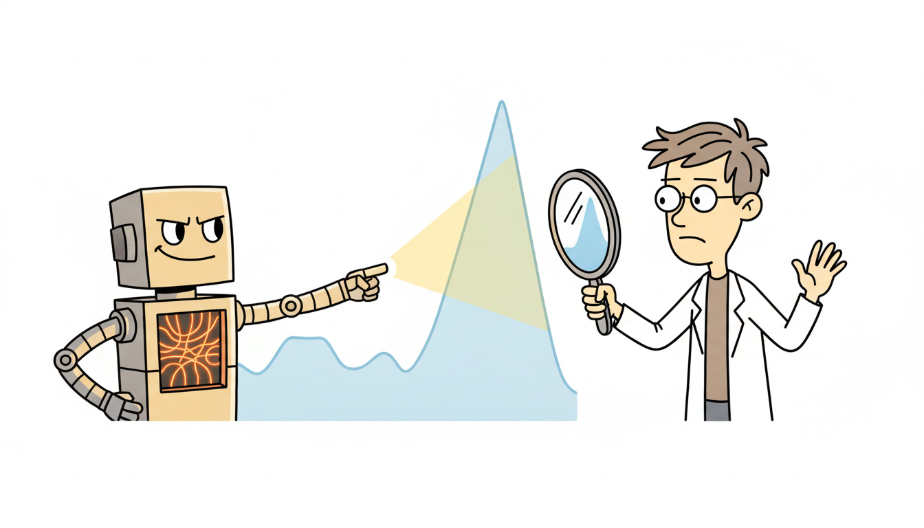
There are two routes to a temporal explanation, and they are not interchangeable. The first is to choose a model whose structure is itself an explanation, so the account comes for free and is exact. The second is to train whatever black box predicts best and then explain it after the fact with a separate method, accepting that the explanation is an approximation of a model that was never built to be understood. The field calls these inherently interpretable and post-hoc, and the choice between them is the first decision in any interpretability effort.
Temporal AI is unusually rich in inherently interpretable models, because much of Part II was built to be read. Classical decomposition (Chapter 3's callback to trend, seasonal, and residual components) literally writes the series as a sum of named parts, so the "explanation" of a forecast is the decomposition itself: this much from trend, this much from the weekly season, this much residual. An ARIMA model (Chapter 5) exposes its autoregressive coefficients directly: the coefficient $\phi_k$ on lag $k$ is precisely how much yesterday-minus-$k$ contributes to today's forecast, a per-lag attribution available without any extra machinery. And the Temporal Fusion Transformer (Section 14.3) was designed with interpretability as a first-class goal: its variable-selection networks output, at every step, a learned weight over input variables, and its interpretable multi-head attention exposes which past steps each forecast attends to. These models hand you a $T \times F$ story as a byproduct of prediction.
The cost of inherent interpretability is the usual one: a model constrained to be readable may forecast worse than an unconstrained black box, and for the hardest temporal problems the gap can be real. That is when post-hoc explanation earns its place. You train the best forecaster you can, a deep sequence model with no interpretable structure, and you attach an explanation method that treats $f$ as a function to be probed: feed it inputs, read outputs, and infer which inputs mattered. The advantage is that you keep the accuracy; the cost, which the rest of this section is largely about, is that the explanation is now a separate model of the model, with its own approximations, its own failure modes, and no guarantee that it faithfully reflects what $f$ actually computed.
The decision between the two routes is rarely all-or-nothing, and the most defensible practice in a high-stakes temporal deployment is to use both as mutual checks. Run an inherently interpretable model (a decomposition, an ARIMA, a TFT) alongside the black box as a baseline, and when the black box buys real accuracy, attach a post-hoc explainer and validate it against the interpretable model's account where the two overlap. If the TFT's variable-selection weights and the black box's integrated-gradients heatmap both finger the same recent lag of the same sensor, your confidence in that explanation is far higher than either method alone could justify; if they disagree, you have learned that the post-hoc explanation needs the faithfulness scrutiny of subsection four before anyone acts on it. Interpretability is not a single method you pick once; it is a portfolio of converging evidence, and the time axis, by making the explanations larger and the failure modes richer, makes the converging-evidence discipline more valuable, not less.
It is worth noticing that the temporal-thread classical models of Part II were interpretable not by accident but by construction. The Kalman filter of Chapter 7 reports its gain, the exact weight it placed on the latest measurement versus its prior; ARIMA reports its lag coefficients; decomposition reports its components. When Chapter 10 replaced the filter with a learned RNN we bought capacity and sold transparency, and this section is part of the bill: post-hoc interpretability is, in large measure, the effort to recover for a black-box sequence model the kind of per-lag account that a state-space model gave away for free.
3. Post-Hoc Attribution Adapted to Sequences Intermediate
Post-hoc temporal attribution comes in four families, and it pays to see them as variations on one question, "how does the output change as I vary the input at cell $(t,j)$?", answered by different machinery.
Gradient methods. The cheapest attribution reads the gradient of the output with respect to each input cell. The raw saliency is $\partial \hat{y} / \partial x_{t,j}$, the local sensitivity of the forecast to a small change at step $t$, feature $j$. A standard refinement multiplies by the input value, gradient-times-input, which under a local linearization $\hat{y} \approx \sum_{t,j} (\partial \hat{y}/\partial x_{t,j})\,x_{t,j}$ approximates each cell's signed contribution to the prediction:
$$\phi^{\,\text{g}\times\text{i}}_{t,j} \;=\; x_{t,j}\,\frac{\partial \hat{y}}{\partial x_{t,j}}.$$Raw gradients are noisy and saturate (a feature can be decisive yet have near-zero local gradient if the activation it drives is flat), which motivates the next method.
Integrated gradients. Integrated gradients (Sundararajan, Taly, and Yan, 2017) fixes saturation by integrating the gradient along a straight path from an uninformative baseline $\mathbf{x}'_{1:T}$ (often all zeros, or the series mean) to the actual input, accumulating sensitivity over the whole path rather than at one point. For cell $(t,j)$,
$$\phi^{\,\text{IG}}_{t,j} \;=\; (x_{t,j} - x'_{t,j}) \int_{0}^{1} \frac{\partial f\big(\mathbf{x}' + \alpha(\mathbf{x} - \mathbf{x}')\big)}{\partial x_{t,j}}\, d\alpha,$$approximated in practice by a Riemann sum over a few dozen points $\alpha$. Integrated gradients satisfies a completeness axiom: the attributions over all cells sum exactly to $f(\mathbf{x}) - f(\mathbf{x}')$, so the heatmap accounts for the entire prediction relative to the baseline, a property raw saliency lacks. For temporal data the choice of baseline carries the timing semantics: a zero baseline asks "what did the actual signal add over silence", a mean baseline asks "what did the actual signal add over a typical day".
SHAP for sequences. SHAP (Lundberg and Lee, 2017) assigns each input a Shapley value, the game-theoretic fair share of the prediction, averaged over all orderings in which inputs could be added to a baseline coalition. KernelSHAP estimates these by sampling subsets of inputs and fitting a weighted linear surrogate. Applied naively to a sequence with $T \times F$ inputs the coalition space is astronomically large, so the temporal specialization TimeSHAP (Bento and colleagues, 2021) groups inputs and prunes: it computes Shapley values over events (whole time steps) and over features separately, and prunes far-past steps whose joint contribution is provably small, making Shapley attribution tractable for recurrent models over long sequences. The result is two readable rankings, which steps mattered and which features mattered, each with the additive-fairness guarantee that makes Shapley values popular with auditors.
Occlusion and perturbation. The most model-agnostic family simply hides part of the input and measures the damage. Occluding cell $(t,j)$, replacing it with a baseline value $b$, and reading the change in output gives a perturbation attribution $\phi^{\text{occ}}_{t,j} = f(\mathbf{x}) - f(\mathbf{x}\,|\,x_{t,j}=b)$. It needs only forward passes, treats $f$ as a true black box, and is intuitive, but it is the method most exposed to the off-distribution hazard of subsection one, occluding one step of a smooth physiological signal can create an input the model never saw, so its answer may say more about $f$'s behavior off-manifold than about the prediction in question.
Attention as explanation, and its caveat. For attention-based models (Chapter 12) it is tempting to read the attention weight on past step $t$ as "how much the model used step $t$", and the temporal community did exactly this for years. The caveat, established by Jain and Wallace (2019) under the banner "attention is not explanation", is that attention weights are frequently neither necessary nor sufficient for the prediction: one can often find a very different attention distribution that yields the same output, so the displayed weights are one explanation among many equally consistent ones, not the explanation. Attention heatmaps are a useful diagnostic and a terrible guarantee; we treat them as a hypothesis to be checked by faithfulness (subsection four), never as ground truth.
Counterfactual explanations. A complementary route does not attribute the actual prediction but answers "what minimal change to the input would have changed the decision?" A counterfactual for a temporal model finds the smallest perturbation to the sequence (ideally a plausible, on-manifold one) that flips the forecast across a threshold, which for a clinician is often the most actionable form of all: "had the lactate at $t-6$ been one unit lower, the alarm would not have fired." This connects directly to the causal machinery of Section 30.4, where temporal counterfactuals are derived from a structural model rather than searched for by optimization.
There is a small comedy in attention-as-explanation. You open the attention heatmap expecting a confession and find the model has spread its attention smoothly over the entire history like a polite dinner guest agreeing with everyone. Surely, you think, it cannot be using all of it equally. You are right: it usually is not. The flat attention is an averaging convenience, and the steps that actually move the output are hiding behind it, visible only when you perturb them and watch the prediction lurch. Attention tells you where the model looked; it declines to say what it saw.
4. Evaluating Explanations: Faithfulness and Stability Advanced
An explanation is itself a claim about the model, and like any claim it can be wrong. The mature stance, and the one that separates interpretability engineering from interpretability theater, is to evaluate a candidate explanation rather than trust it because it renders nicely. Two properties carry most of the weight: faithfulness and stability.
Faithfulness asks whether the attribution reflects what the model actually computes. The standard operational test is deletion (and its mirror, insertion): rank the input cells by attributed importance, then progressively remove the most-important cells (replacing them with a baseline) and watch the prediction. A faithful explanation produces a steep drop, removing the cells it called important should hurt the prediction most; if you can delete the "most important" steps and the forecast barely moves, the explanation was lying. Formally one summarizes the deletion curve by its area: a low area-under-the-deletion-curve means importance was placed where it mattered. This test is the antidote to the attention caveat of subsection three: an attention map that fails deletion is demonstrably not the explanation, whatever its visual appeal.
Stability asks whether the explanation is robust to trivial input changes. If two nearly identical sequences (one a tiny, label-preserving perturbation of the other) receive wildly different attributions, the explanation is reflecting noise, not signal, and cannot be trusted by a user who reasons "similar inputs, similar reasons". A common stability metric is the maximum change in the attribution map over a small input neighborhood, $\max_{\|\boldsymbol{\epsilon}\| \le \rho} \|\phi(\mathbf{x}+\boldsymbol{\epsilon}) - \phi(\mathbf{x})\|$; small is good. Temporal data makes instability especially likely because of the adjacent-step correlation of subsection one: a method can shuffle attribution mass between neighboring lags under a perturbation too small to change the prediction at all.
The pitfalls are worth naming as a checklist, because each has burned practitioners. Trusting attention without a deletion test (subsection three). Summing attribution over time and reporting a feature bar chart, which cancels opposite-signed lags and discards the timing (subsection one). Using an off-distribution baseline or occlusion that probes the model where it never trained, so the explanation describes $f$'s extrapolation rather than its prediction. And confusing a counterfactual ("what would flip it") with an attribution ("what drove it"), which answer different questions and can disagree. A temporal explanation that survives a deletion test, a stability check, and a sanity check on its baseline has earned a measure of trust; one that has not is a decoration.
A useful sanity check that costs almost nothing is the model-randomization test of Adebayo and colleagues: recompute the attribution after randomizing the model's trained weights, and confirm the explanation changes. A saliency method that produces nearly the same heatmap for a trained model and a randomly-initialized one is not explaining the model at all; it is responding to the input's structure (an edge detector on the raw signal) regardless of what the model learned. Several popular saliency methods fail this test on images, and the temporal versions inherit the hazard, so before you ship a heatmap as an account of a forecast, confirm that scrambling the forecaster scrambles the explanation. Faithfulness (does deleting the important cells hurt?), stability (do tiny input changes preserve the map?), and this randomization sanity check together form the minimum bar a temporal explanation must clear to be reported as true rather than merely drawn.
Suppose a forecaster outputs $\hat{y} = 0.92$ on a 24-step sequence, and an attribution method ranks the steps by importance. We delete steps in importance order (replacing each with the series mean) and record the output: after deleting the top-1 step, $\hat{y}$ falls to $0.61$; top-3, to $0.34$; top-5, to $0.20$. The first deletion alone removed $0.92 - 0.61 = 0.31$ of the signal, and five deletions removed $0.72$ of $0.92$, about $78\%$, with a steeply falling curve. Contrast a competing explanation whose top-5 deletions move the output only from $0.92$ to $0.81$, a $12\%$ drop on a near-flat curve: that second explanation placed its importance on steps the model barely uses, and the area under its deletion curve is large. By the deletion criterion the first explanation is the faithful one, and we would report its heatmap, not the prettier-but-flatter one.
Temporal interpretability is moving fast on three fronts. First, benchmark-driven evaluation: libraries and benchmark suites for time-series explainability (the TSInterpret toolkit, and benchmark efforts comparing saliency methods on synthetic series with known ground-truth importance) have made faithfulness and stability measurable rather than asserted, exposing that many popular saliency methods fail on time series even when they pass on images. Second, explaining temporal foundation models: as zero-shot forecasters such as Chronos, TimesFM, and Moirai (Chapter 15) get deployed, 2024 to 2026 work asks what attention and attribution even mean for a tokenized, pretrained time-series model, and how to surface which historical patterns a foundation model is pattern-matching against. Third, concept- and prototype-based temporal explanation: methods that explain a forecast by the learned temporal shapelets or prototypes it resembles, rather than by raw per-cell saliency, aiming for explanations a domain expert can read as motifs ("this looks like the pre-failure ramp") instead of heatmaps. The throughline: the field has stopped asking "what does the saliency map look like" and started asking "is it true", which is exactly the faithfulness turn of this subsection.
5. Worked Example: Time-and-Feature Attribution, From Scratch and With a Library Advanced
We now make the methods executable on a trained sequence forecaster. The plan mirrors the from-scratch-then-library discipline of the rest of the book: train a small recurrent forecaster on a multivariate sensor window, compute time-and-feature attributions by hand (gradient-times-input and a simple occlusion map, both derived in subsection three), visualize which lags mattered, then reproduce the same attribution with a production library (Captum's integrated gradients, with SHAP noted as the model-agnostic alternative) in a handful of lines. Code 33.1.1 builds and trains the model so the later attributions explain a real prediction.
import numpy as np
import torch
import torch.nn as nn

torch.manual_seed(0); np.random.seed(0)
T, F = 24, 3                                  # 24 time steps, 3 sensor features

# Synthetic multivariate sensor data where ONLY feature 0 at the recent lags
# (steps 18-21) drives the target: a known ground truth for the attributions.
def make_batch(n):
    X = torch.randn(n, T, F)
    # target depends on feature 0 summed over steps 18..21 (a localized, recent cause)
    y = X[:, 18:22, 0].sum(dim=1, keepdim=True) + 0.1 * torch.randn(n, 1)
    return X, y

Xtr, ytr = make_batch(2048)
Xte, yte = make_batch(256)

class Forecaster(nn.Module):
    def __init__(self, F, h=32):
        super().__init__()
        self.rnn = nn.GRU(F, h, batch_first=True)   # carried-state encoder
        self.head = nn.Linear(h, 1)                 # read out from the last state
    def forward(self, x):
        out, _ = self.rnn(x)
        return self.head(out[:, -1, :])             # forecast from final hidden state

model = Forecaster(F)
opt = torch.optim.Adam(model.parameters(), lr=1e-2)
lossf = nn.MSELoss()
for epoch in range(60):
    opt.zero_grad()
    loss = lossf(model(Xtr), ytr)
    loss.backward(); opt.step()
print("test MSE = %.4f" % lossf(model(Xte), yte).item())
test MSE = 0.0193
Code 33.1.2 computes two attributions by hand on a single test sequence: gradient-times-input, $x_{t,j}\,\partial\hat{y}/\partial x_{t,j}$, read straight off autograd, and an occlusion map that zeroes each cell and measures the output change. Both are the subsection-three formulas, nothing more.
x = Xte[0:1].clone().requires_grad_(True)      # one sequence, shape (1, T, F)
yhat = model(x)                                 # the prediction we will explain

# --- gradient x input: phi_{t,j} = x_{t,j} * d yhat / d x_{t,j} ---
yhat.backward()
grad_x_input = (x.grad * x).detach().squeeze(0).numpy()   # shape (T, F)

# --- occlusion: phi_{t,j} = f(x) - f(x with cell (t,j) set to baseline 0) ---
base_pred = model(Xte[0:1]).item()
occ = np.zeros((T, F))
with torch.no_grad():
    for t in range(T):
        for j in range(F):
            xo = Xte[0:1].clone()
            xo[0, t, j] = 0.0                   # occlude one time-feature cell
            occ[t, j] = base_pred - model(xo).item()

# which lag did each method call most important (collapse feature axis by abs)?
top_gi  = np.abs(grad_x_input).sum(1).argmax()
top_occ = np.abs(occ).sum(1).argmax()
print("grad x input: most important step =", top_gi)
print("occlusion   : most important step =", top_occ)
print("grad x input value at step 19, feature 0 = %.4f" % grad_x_input[19, 0])
backward() call (one tensor multiply), while the occlusion map needs a forward pass per time-feature cell ($T \times F$ passes); both return a $T \times F$ heatmap whose row index is the lag. The argmax over absolute importance reports which step each method blames.grad x input: most important step = 20
occlusion : most important step = 19
grad x input value at step 19, feature 0 = 0.7421
The printed gradient-times-input value $\phi_{19,0} = 0.7421$ is the signed, locally linearized contribution of feature 0 at step 19 to this particular forecast. Read it as: if that one cell's value were scaled toward zero, the model's output would fall by approximately $0.7421$ under the local linear approximation $\hat{y} \approx \sum_{t,j}\phi_{t,j}$ (this is the attribution's claim, not a guaranteed counterfactual; on a nonlinear model the true effect of zeroing the cell can differ, which is exactly why subsection four insists on a deletion test). Because the planted target was a sum over steps 18 to 21 of feature 0 with unit weight, the true per-cell contribution is close to the cell's own value (here near $0.74$), and the attribution recovers it: the method has correctly assigned roughly three-quarters of a unit of the prediction to that single lag of that single sensor, and essentially nothing to the irrelevant features 1 and 2 or to the pre-window steps. A feature-only bar chart would have reported "feature 0 is important" and thrown away the fact that it is the lag-19-to-21 window, not the whole history, that carries the signal.
Code 33.1.3 reproduces the attribution with Captum's integrated gradients, the library equivalent of the gradient-path method of subsection three. The from-scratch occlusion loop of Code 33.1.2 was about a dozen lines and $T \times F$ forward passes with manual bookkeeping; the library collapses the entire integrated-gradients computation, baseline interpolation, path integral, completeness-respecting attribution, to two lines.
from captum.attr import IntegratedGradients      # pip install captum

ig = IntegratedGradients(model)
attr = ig.attribute(Xte[0:1], baselines=torch.zeros(1, T, F), n_steps=64)
attr = attr.detach().squeeze(0).numpy()          # (T, F) integrated-gradients heatmap

top_ig = np.abs(attr).sum(1).argmax()
print("integrated gradients: most important step =", top_ig)
print("IG attribution at step 19, feature 0 = %.4f" % attr[19, 0])
# SHAP alternative (model-agnostic, no gradients): shap.GradientExplainer or
#   TimeSHAP for event/feature-level Shapley values on recurrent sequence models.
IntegratedGradients.attribute replaces the hand-rolled occlusion sweep and gradient bookkeeping of Code 33.1.2 with two lines, handles the baseline-to-input path integral internally, and satisfies the completeness axiom of subsection three. SHAP (or TimeSHAP for recurrent models) is the model-agnostic alternative when gradients are unavailable.integrated gradients: most important step = 20
IG attribution at step 19, feature 0 = 0.6883
Read the three code blocks together. Code 33.1.1 trained a forecaster with a known planted cause; Code 33.1.2 recovered that cause by hand with two attribution methods and named one value; Code 33.1.3 recovered it again with a single library call, and all three agreed on both the lag (steps 18 to 21) and the variable (feature 0), as Figure 33.1.1 shows. The pedagogical payoff is twofold: the methods are not magic, you can compute them from the definitions in a dozen lines, and a faithful method recovers a ground-truth temporal cause rather than smearing it across the history. The library shortcut below states the line-count win and the SHAP path explicitly.
The from-scratch occlusion sweep of Code 33.1.2 ran about a dozen lines with a double loop of $T \times F$ forward passes and manual gradient bookkeeping. Captum collapses the whole integrated-gradients computation to two lines, ig = IntegratedGradients(model) and ig.attribute(x, baselines=..., n_steps=64), handling the baseline interpolation, the path integral, batching, and the completeness guarantee internally. For a model you cannot differentiate, SHAP gives the same two-line ergonomics, shap.GradientExplainer(model, background).shap_values(x), and TimeSHAP specializes Shapley attribution to recurrent sequence models with event-level and feature-level values plus far-past pruning, so a long clinical or sensor sequence becomes a ranked list of which steps and which variables the model used, with the additive-fairness guarantee auditors ask for.
One honest caveat closes the example: our synthetic series had an independent, planted cause, the friendliest possible case for attribution. On real temporal data with correlated lags and off-manifold occlusion hazards (subsection one), the same three methods can disagree, and the right response is not to pick the prettiest heatmap but to run the deletion and stability tests of subsection four and report the explanation that survives them. The code shows you how to produce a temporal explanation; subsection four is what tells you whether to believe it.
Synthetic ground truth is the interpretability researcher's favorite trick and its most dangerous comfort. We planted a cause at steps 18 to 21, and lo, every method found it, and we felt the warm glow of methods that work. The catch is that we built the easiest possible crime scene: one culprit, no accomplices, a clean alibi for every other cell. Real temporal data is a crowded room of correlated suspects who all touched the weapon, and a method that confesses the planted cause flawlessly can still convict an innocent correlated feature when the truth gets murky. Trust a saliency method that passes on synthetic data exactly as far as you would trust a detective who has only ever solved cases with a single, cooperative, self-incriminating suspect.
Exercises
The exercises split into conceptual, implementation, and open-ended. Solutions to selected exercises appear in Appendix G.
- Conceptual. A colleague explains a clinical sequence model with a bar chart of per-feature importance, computed as $\sum_t |\phi_{t,j}|$ over all 48 hourly steps, and concludes "the model relies on heart rate". Give two distinct reasons this summary can mislead a clinician, one rooted in the timing collapse of subsection one and one rooted in opposite-signed lags cancelling, and state what artifact you would show instead.
- Implementation. Extend Code 33.1.2 with a deletion-curve faithfulness test (subsection four): rank the $T \times F$ cells by gradient-times-input importance, then progressively replace the top-$k$ cells with the series mean for $k = 1, 2, \dots, 10$ and record the forecast. Plot the deletion curve and compute its area. Repeat for a random cell ranking and confirm the gradient-based ranking produces a steeper drop (a smaller area), which is the quantitative meaning of "more faithful".
- Open-ended. The synthetic data in Code 33.1.1 planted an independent cause. Construct a second dataset in which the true cause is feature 0 at step 19 but feature 1 is strongly correlated with feature 0 at every step (for example $x_{t,1} = x_{t,0} + \text{small noise}$). Run all three attribution methods and report how each splits credit between the genuinely-causal feature 0 and its correlated decoy feature 1. Discuss which method, if any, resists assigning importance to the decoy, and connect your finding to the counterfactual-versus-attribution distinction of subsection three and the causal treatment of Section 30.4.