"For three years I reported that ice cream sales predict drownings with a p-value to die for, and they promoted me. Then someone whispered the word 'summer' and my entire career collapsed into a confounder. I can forecast anything; what I cannot do, it turns out, is tell you what to push on."
An Algorithm Trying to Tell Correlation From Genuine Cause
Everything earlier in this book learned to predict the future from the past. This section asks a harder question that prediction alone can never answer: which past variables actually cause the future, in the sense that intervening on them would change it. A forecaster that exploits the correlation between ice cream sales and drownings will score beautifully and advise catastrophically, because both are driven by a hidden third variable, the season. Causal discovery for time series is the project of recovering, from observational multivariate series alone, a graph whose edges $X^i_{t-\tau} \to X^j_t$ mean genuine lagged causal influence rather than mere predictability. We start by sharpening exactly why Granger causality (which you met as a predictive test in Section 6.2) measures predictability, not causation, and what assumptions would be needed to close the gap. We then build the modern toolkit: constraint-based discovery with PCMCI and PCMCI+ and its tigramite implementation, which test conditional independence across time lags while controlling autocorrelation and high dimensionality; neural-Granger networks and functional causal models (VAR-LiNGAM, additive-noise) as score-based alternatives; and the assumptions each one rests on (causal sufficiency, stationarity, faithfulness). We catalog the pitfalls that quietly invalidate discovered graphs (hidden confounders, and the way subsampling or temporal aggregation, the very resampling of Section 2.2, can manufacture spurious arrows). Finally we generate data from a known lagged graph, recover it twice (a from-scratch lagged conditional-independence test and tigramite PCMCI), and compare both to ground truth. You leave able to run, read, and distrust a causal-discovery result with the right amount of suspicion.
In Section 30.1 we framed temporal reasoning as the move from pattern recognition to structured inference about how a system's variables relate over time. This section takes the first concrete step into causality: discovering the causal structure itself. The motivating gap is one every practitioner eventually hits. A model that forecasts well tells you what will happen if the world keeps behaving as it did; it does not tell you what would happen if you reached in and changed something. A demand forecaster can predict that low prices accompany high sales without telling you whether cutting prices will raise sales or whether both move together because of a promotion you did not record. The first question is predictive (the subject of Parts II through V); the second is causal, and answering it from data alone is the subject of causal discovery. We use the unified notation of Appendix A: a multivariate series $\mathbf{X}_t = (X^1_t, \dots, X^N_t)$ of $N$ component series observed over time $t$, and a target causal graph $\mathcal{G}$ whose nodes are the lagged components $X^i_{t-\tau}$.
Why does this deserve its own section rather than a footnote to forecasting? Because the entire downstream value of an intelligent temporal system, the ability to plan, to intervene, to attribute, to act (the agents of Section 30.3 and the world models of Chapter 29) rests on having a causal model, not merely a predictive one. A policy that optimizes against a purely predictive model will happily exploit correlations that evaporate the instant it acts on them, the temporal analogue of the classic confounding trap. Getting the causal graph approximately right, and knowing exactly which assumptions you bought it with, is what separates a system that reasons from one that merely pattern-matches with confidence.
The competencies this section installs are four: to state precisely why Granger predictability falls short of causation and what closes the gap; to run a constraint-based discovery procedure (PCMCI) and read its lagged conditional-independence logic; to recognize the assumption set (sufficiency, stationarity, faithfulness) that every discovery method silently requires; and to recover a known graph from synthetic data with both a hand-built test and a library, comparing both to the truth. These are the load-bearing skills for every causal claim a temporal system will ever make.
1. From Prediction to Cause: Why Granger Predictability Is Not Causation Beginner
Recall the Granger test of Section 6.2. We said $X$ Granger-causes $Y$ if the past of $X$ improves the prediction of $Y$ beyond what the past of $Y$ alone achieves: formally, if $\operatorname{Var}[Y_t \mid Y_{
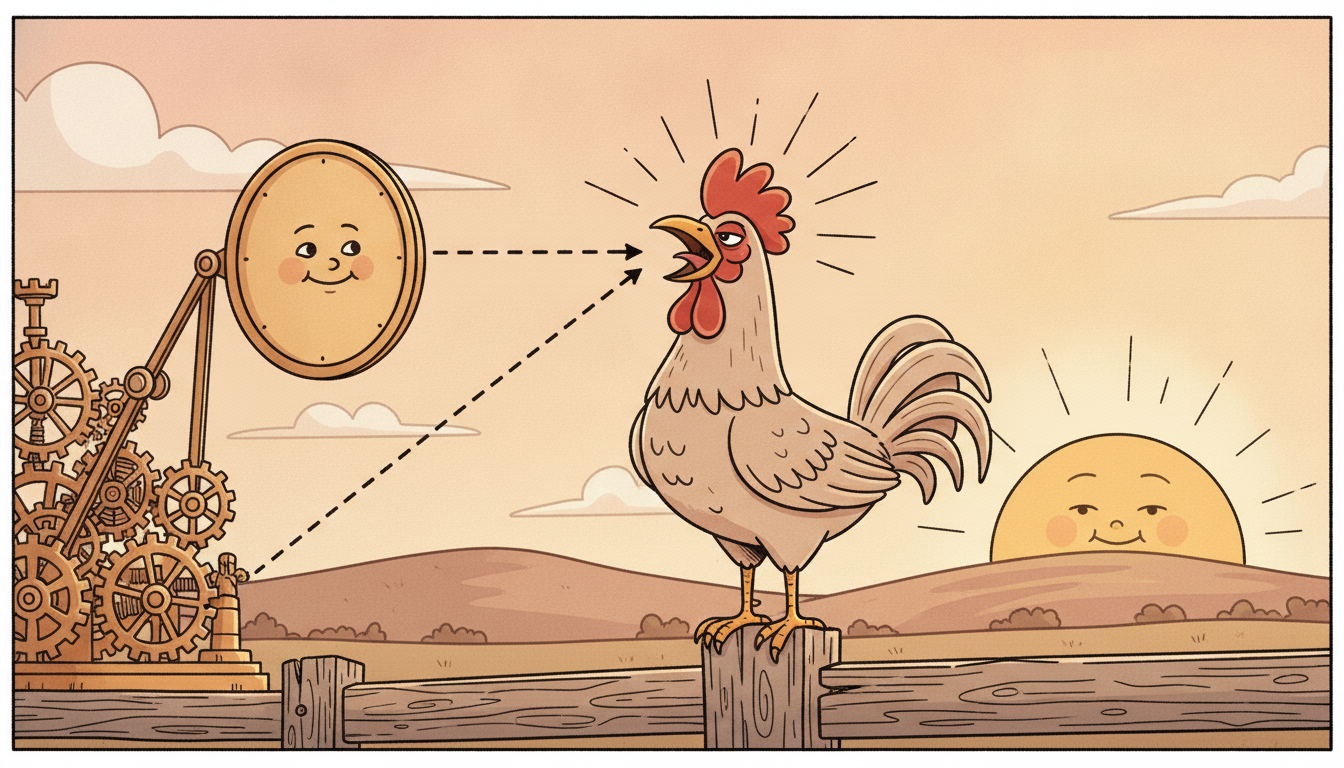
The word "cause" in "Granger cause" is a historical misnomer that has misled generations of practitioners. The Granger criterion tests whether $X$'s past carries information about $Y$'s future that $Y$'s own past does not. Three distinct worlds produce that signal, and only one of them is genuine causation. First, $X$ really does cause $Y$. Second, a hidden common driver $Z$ causes both $X$ and $Y$ with $X$ leading (the ice cream and drownings of the epigraph, both driven by summer heat $Z$): $X$ predicts $Y$ while changing $X$ does nothing. Third, selection or conditioning on a common effect opens a spurious dependence. Granger's predictive test cannot tell these worlds apart from a bivariate series, because predictability is symmetric to the data-generating story in a way that causation is not.
To say what causation is we need a structural model, not just a predictive one. A structural causal model for a time series writes each component as a deterministic function of its true causal parents (lagged variables) plus an independent noise term:
$$X^j_t = f_j\!\left(\, \big\{ X^i_{t-\tau} : (i,\tau) \in \mathrm{pa}(j) \big\} \,\right) + \varepsilon^j_t, \qquad \varepsilon^j_t \perp\!\!\!\perp \varepsilon^k_s \ \ \text{for } (j,t)\neq(k,s),$$where $\mathrm{pa}(j)$ is the set of lagged causal parents of $X^j_t$ and the noises $\varepsilon^j_t$ are mutually independent. The crucial extra content over a predictive model lives in the word intervene: the causal graph licenses the interventional claim that setting $X^i_{t-\tau}$ to a chosen value (the $\operatorname{do}$-operator of Pearl) propagates through $f_j$ to change $X^j_t$, whereas a purely observational correlation carries no such guarantee. Time gives causality one free gift the static case lacks, namely the arrow of time itself: a cause cannot follow its effect, so every causal edge must point from a strictly earlier (or, for instantaneous effects, contemporaneous) variable to a later one, which rules out half the candidate edges before any test is run. This temporal priority is the single feature that makes time-series discovery more tractable than discovery on static data.
Granger causality asks "does $X$'s past reduce my uncertainty about $Y$'s future?". Three different causal worlds, $X \to Y$, a hidden confounder $Z \to X$ and $Z \to Y$, and selection on a common effect, all answer "yes". The predictive test cannot distinguish them, because it never considers what would happen under intervention. To recover causation you must add structure: either control for the right conditioning variables so that only genuine causal links survive (the constraint-based route of subsection two), or assume a functional form whose asymmetry breaks the tie (the score-based route of subsection three). There is no assumption-free path from a correlation, however predictive, to a cause.
This is why "causal discovery" is a different enterprise from forecasting and not merely a fancier version of it. Discovery's goal is the graph $\mathcal{G}$, and the graph is judged not by how well it predicts but by whether its edges survive the right conditioning. The remainder of this section is two families of methods for recovering that graph, the assumptions they need, and the ways they fail.
2. Constraint-Based Discovery: PCMCI, PCMCI+, and tigramite Intermediate
The constraint-based family recovers a causal graph by a disciplined sequence of conditional-independence (CI) tests. The governing idea, inherited from the PC algorithm for static data, is the faithfulness assumption: two variables are conditionally independent given a separating set if and only if there is no causal edge between them in the graph. So if we can find, for a candidate link $X^i_{t-\tau} \to X^j_t$, some conditioning set $\mathbf{S}$ that renders the two conditionally independent, $X^i_{t-\tau} \perp\!\!\!\perp X^j_t \mid \mathbf{S}$, we delete the link; if no such set exists, we keep it. The art is choosing $\mathbf{S}$ correctly, because the naive PC approach applied to time series stumbles on two facts unique to temporal data.
The first stumbling block is autocorrelation: each series is correlated with its own past, so a link $X^i_{t-\tau} \to X^j_t$ can look significant simply because both endpoints share the strong autocorrelated background of $X^j$, inflating false positives. The second is high dimensionality: with $N$ series and a maximum lag $\tau_{\max}$, there are $N \cdot \tau_{\max}$ candidate parents for each target, and the conditioning sets explode combinatorially, destroying the power of the CI tests. PCMCI, introduced by Runge and colleagues, is engineered precisely around these two problems, and it does so in two stages.
- PC$_1$ (condition selection): for each target $X^j_t$, run a Markov-blanket-style iterative filter that identifies a small set of the strongest lagged conditions $\hat{\mathcal{P}}(X^j_t)$, pruning the combinatorial candidate set down to the genuinely relevant parents. This stage controls dimensionality by never conditioning on more than a compact, adaptively chosen set.
- MCI (momentary conditional independence): for each surviving candidate link $X^i_{t-\tau} \to X^j_t$, test independence while conditioning on both the parents of the target $\hat{\mathcal{P}}(X^j_t)$ and the parents of the lagged source $\hat{\mathcal{P}}(X^i_{t-\tau})$. Conditioning on the source's own parents is the trick that controls autocorrelation: it removes the shared autocorrelated background that would otherwise fake a link.
The MCI test statistic for a link is therefore a conditional independence of the form
$$X^i_{t-\tau} \ \perp\!\!\!\perp\ X^j_t \ \ \big|\ \ \hat{\mathcal{P}}(X^j_t) \setminus \{X^i_{t-\tau}\},\ \ \hat{\mathcal{P}}(X^i_{t-\tau}),$$and the link is kept in $\mathcal{G}$ if and only if this independence is rejected at significance level $\alpha$. The choice of CI test is modular: partial correlation (ParCorr) for linear Gaussian dependencies, a kernel-based test (GPDC, Gaussian-process distance correlation) or conditional mutual information (CMIknn, a $k$-nearest-neighbor estimator) for nonlinear dependencies. The original PCMCI recovers lagged links and is provably consistent under its assumptions; PCMCI+ (Runge, 2020) extends it to also discover contemporaneous (zero-lag) links by adding a momentary-CI phase among same-time variables, which matters whenever your sampling rate is coarser than the true causal delay so that genuine causes appear instantaneous. Both are implemented in the open-source tigramite toolkit, which is the reference software for the field and the one we use in subsection five.
| Stage | What it does | Problem it solves |
|---|---|---|
| PC$_1$ condition selection | iteratively prune candidate parents to a compact $\hat{\mathcal{P}}(X^j_t)$ | high dimensionality / combinatorial conditioning sets |
| MCI test | test each link conditioning on parents of both endpoints | autocorrelation inflating false positives |
| PCMCI+ extra phase | add contemporaneous (zero-lag) link discovery | true causes appearing instantaneous under coarse sampling |
| CI test choice | ParCorr / GPDC / CMIknn | linear vs nonlinear dependence |
The payoff of this engineering is statistical: PCMCI controls the false-positive rate at the nominal $\alpha$ far better than naive lagged-regression or vanilla PC on autocorrelated data, and it retains detection power as $N$ and $\tau_{\max}$ grow, which is exactly the regime, dozens of climate or sensor channels with long memory, where causal discovery is most wanted. That same engineering is why we reach for the library rather than hand-rolling the full procedure in production; subsection five shows the from-scratch single-link test that PCMCI generalizes.
The cleverest part of MCI has a faintly self-referential charm: to decide whether $X$ truly causes $Y$, it conditions on $X$'s own causal parents. The intuition is that if a hidden-but-recorded driver was feeding $X$, conditioning on $X$'s parents soaks up the autocorrelated portion of $X$ that the driver was responsible for, so any leftover dependence with $Y$ is more likely to be $X$'s own doing. It is the statistical equivalent of asking a suspect to first account for everyone who influenced them, and only then judging whether what remains points to the crime. It does not catch unrecorded confounders (nothing observational can), but it is remarkably effective against the recorded ones.
3. Other Approaches: Neural Granger, Score-Based and Functional Causal Models Intermediate
Constraint-based discovery is not the only route to the graph. Two other families trade the CI-testing machinery for assumptions about functional form, and each buys something the constraint-based view cannot.
Neural Granger causality. Classical Granger tests fit a linear vector-autoregression and ask whether a coefficient block is zero. Neural-Granger methods (Tank and colleagues, 2018 onward) replace the linear VAR with a neural network, one multilayer or recurrent network per target series, and read causality off structured sparsity in the input weights. If the network predicting $X^j_t$ assigns near-zero weight to all lagged values of $X^i$ (enforced by a group-lasso penalty on the input layer, one group per candidate source series), then $X^i$ does not neural-Granger-cause $X^j$. This captures nonlinear lagged dependence that a linear Granger test would miss, at the price of the same predictive-versus-causal gap as classical Granger: it still measures predictability, now nonlinear, and still cannot by itself rule out a hidden confounder. Its strength is flexibility and scalability to many series; its weakness is that it inherits Granger's interpretation caveat in full.
Functional causal models. The score-based / functional family makes the opposite bet: assume a restricted functional form whose asymmetry identifies causal direction even without an interventional experiment. The two canonical instances for time series are:
- VAR-LiNGAM (linear non-Gaussian acyclic model, the time-series extension of LiNGAM): assume the structural equations are linear with non-Gaussian independent noise. The remarkable identifiability result is that non-Gaussianity breaks the direction symmetry that defeats Gaussian methods: the true causal order is the unique one for which the residuals are independent, recoverable by independent component analysis. This fixes a complete directed graph including contemporaneous links, where constraint-based methods would leave some edges unoriented.
- Additive-noise models (ANM): assume $X^j_t = f_j(\text{parents}) + \varepsilon^j_t$ with $f_j$ possibly nonlinear and $\varepsilon^j_t$ independent of the parents. The identifying signal is that for the true causal direction the residual is independent of the cause, whereas for the wrong direction it is not (generically). This handles nonlinearity that LiNGAM's linearity cannot.
Each method rests on a precise assumption set, and being able to recite which assumption each one buys is the single most useful skill in reading a discovery result. Three assumptions recur across every method in this section.
$$\underbrace{\text{causal sufficiency}}_{\text{no hidden common causes}} \quad+\quad \underbrace{\text{stationarity}}_{\text{the graph and } f_j \text{ do not change over time}} \quad+\quad \underbrace{\text{faithfulness}}_{\text{no exact cancellation hides a true edge}}.$$Causal sufficiency says every common cause of two observed variables is itself observed (no unrecorded confounders); it is the assumption most often violated in practice and the one subsection four dissects. Stationarity says the causal mechanism is fixed across the observation window, so that pooling time points to estimate one graph is valid; a regime change (the drift of Chapter 20) silently breaks it. Faithfulness says the only conditional independences in the data are those forced by the graph structure, so a true edge cannot be hidden by two effects exactly cancelling; it is usually mild but fails on the measure-zero (yet engineering-relevant) cases of perfectly tuned feedback loops. Constraint-based methods lean hardest on faithfulness; functional methods lean hardest on the assumed functional form and noise distribution; all of them assume sufficiency and stationarity unless explicitly extended.
The field is moving fast on exactly the assumptions subsection four shows are fragile. LPCMCI and the related latent-PCMCI variants (Gerhardus and Runge) relax causal sufficiency to discover graphs in the presence of unobserved confounders and selection, returning ancestral graphs with explicit "latent confounder" marks rather than pretending none exist. Regime-PCMCI and change-point-aware discovery attack the stationarity assumption by jointly inferring regimes and a per-regime graph. On the functional side, differentiable causal discovery recasts the whole search as continuous optimization with a smooth acyclicity constraint (the NOTEARS family and its dynamic extension DYNOTEARS, 2020, for time series), and 2024 to 2026 work fuses this with neural structural equations and amortized, transformer-based discovery that learns to output a graph from a series in a single forward pass (for example AVICI-style amortized inference). A recurring 2024 to 2026 theme is benchmarking honesty: the CauseMe platform and tigramite's expanding test suite have made it routine to report discovery on realistic confounded, nonstationary data rather than the toy linear-Gaussian graphs that flatter every method. The practitioner's takeaway: assume your real data violates sufficiency and stationarity, and prefer a method that says so.
4. Pitfalls: Hidden Confounders, Subsampling, and the Limits of Observation Advanced

Every discovered graph is a conditional statement: "if the assumptions hold, these are the causal links." The pitfalls of this subsection are the ways those assumptions silently fail, turning a confident graph into a confident error. Three failure modes dominate, and all three are invisible to the discovery algorithm itself, which is why they must live in the practitioner's head.
Hidden confounders. The violation of causal sufficiency is the deepest pitfall because nothing in observational data can detect or repair it in general. If an unrecorded variable $Z$ drives both $X$ and $Y$, no conditioning set built from observed variables can separate them, so the discovery algorithm reports a spurious edge $X \to Y$ (or $Y \to X$) with full statistical confidence. The ice cream and drownings of the epigraph are the cartoon; the real cases are an unrecorded market-wide shock that makes two stocks appear to drive each other, or an unmeasured patient-acuity variable that makes a treatment appear to cause an outcome it merely correlates with. The only true defenses are external: record the suspected confounder, run an actual intervention, or use a method (LPCMCI) that at least flags the possibility of a latent driver rather than silently orienting the edge.
Subsampling and temporal aggregation. This pitfall is subtler and specifically temporal, and it connects directly to the resampling discussion of Section 2.2. Suppose the true causal delay from $X$ to $Y$ is one step at the system's native sampling rate, but you observe the series subsampled (every other step) or aggregated (summed or averaged into coarser bins). The observed series can then exhibit causal structure that does not exist at the true rate: a clean unidirectional $X \to Y$ at the fine scale can appear as a bidirectional or even reversed link after subsampling, because the intermediate step that carried the influence has been hidden, and aggregation can blur a lagged link into a spurious contemporaneous one. The sampling rate is not a neutral choice of resolution; it is a transformation that can create and destroy causal arrows.
Take a true two-variable system at the native rate with a one-step chain $X_{t-1} \to Y_t$ and $Y_{t-1} \to X_t$ both present (a fast feedback loop), with coefficient $0.8$ each and equal noise. At the native rate, a lag-1 analysis correctly finds both links. Now subsample by keeping only even time indices, so the observed step is two native steps. The two-step transition matrix is $\mathbf{A}^2$ where $\mathbf{A} = \begin{pmatrix} 0 & 0.8 \\ 0.8 & 0 \end{pmatrix}$, giving $\mathbf{A}^2 = \begin{pmatrix} 0.64 & 0 \\ 0 & 0.64 \end{pmatrix}$: at the subsampled rate the cross links vanish and each variable appears to depend only on its own past, so a lag-1 discovery on the subsampled data reports only autodependence and no cross-coupling, erasing the true $X \leftrightarrow Y$ feedback. Halve the sampling rate again and aliasing can resurrect a phantom cross-link with the wrong sign. The lesson is quantitative: the causal graph you recover is a function of the sampling rate, and there is no rate-invariant graph to recover unless you sample at or above the true causal frequency.
The fundamental limit of observation. Underlying both specific pitfalls is a single principled boundary: observational data alone, however abundant, cannot in general identify a unique causal graph. The best a constraint-based method can return is a Markov equivalence class, a set of graphs that are statistically indistinguishable because they imply the same conditional independences. Temporal priority shrinks this class (arrows must respect time) and functional assumptions can shrink it to a single graph (LiNGAM's non-Gaussianity, ANM's additivity), but those are assumptions, not facts read from data, and if they are wrong the unique answer is confidently wrong. The honest stance, and the one a trustworthy temporal system must encode, is that discovery yields hypotheses ranked by plausibility under stated assumptions, and the gold standard for confirming a causal edge remains an intervention (the controlled experiment, the A/B test, the policy change), which is precisely the bridge into the interventional reasoning of Section 30.3.
No causal-discovery algorithm reads causation off data; each reads it off data plus a set of assumptions (sufficiency, stationarity, faithfulness, and often a functional form). When the assumptions hold, the graph is sound; when they fail, the algorithm gives no warning and the graph is confidently wrong. Hidden confounders break sufficiency, regime changes break stationarity, and the sampling rate can manufacture or erase arrows entirely. Treat every discovered edge as a falsifiable hypothesis whose strongest confirmation is an actual intervention, and you will use these tools the way they were meant to be used: to propose causal structure cheaply from observation, then spend expensive experiments only where it matters.
5. Worked Example: Recover a Known Lagged Graph, From Scratch and With tigramite Advanced
We now make the whole section executable. The plan: simulate a three-variable series from a known lagged causal graph, so we have ground truth; recover that graph two ways, first with a from-scratch lagged conditional-independence test built on partial correlation (the atom that PCMCI generalizes), then with tigramite's PCMCI; and compare both recovered graphs to the truth. Code 30.2.1 builds the synthetic data and the from-scratch discovery. The ground-truth graph has three lagged edges: $X^0_{t-1} \to X^1_t$, $X^1_{t-1} \to X^2_t$, and an autodependence $X^0_{t-1} \to X^0_t$, with no edge from $X^2$ into anything (so $X^2$ is a pure sink).
import numpy as np
from scipy import stats

rng = np.random.default_rng(0)
T, tau_max, alpha = 2000, 2, 0.01     # length, max lag tested, significance level

# Ground-truth lagged structural model (the graph we will try to recover):
#   X0_t = 0.7 X0_{t-1}                 + e0   (autodependence)
#   X1_t = 0.6 X0_{t-1}                 + e1   (X0 -> X1 at lag 1)
#   X2_t = 0.5 X1_{t-1}                 + e2   (X1 -> X2 at lag 1)
X = np.zeros((T, 3))
for t in range(1, T):
    X[t, 0] = 0.7 * X[t-1, 0]            + rng.normal(0, 1)
    X[t, 1] = 0.6 * X[t-1, 0]            + rng.normal(0, 1)
    X[t, 2] = 0.5 * X[t-1, 1]            + rng.normal(0, 1)

def partial_corr_test(a, b, Z):
    """Partial correlation of a and b given the columns of Z, with a p-value.
    Regress a and b on Z, correlate the residuals (this is the ParCorr CI test)."""
    if Z.shape[1] == 0:
        r, p = stats.pearsonr(a, b)
        return r, p
    beta_a, *_ = np.linalg.lstsq(Z, a, rcond=None)   # residualize a against Z
    beta_b, *_ = np.linalg.lstsq(Z, b, rcond=None)   # residualize b against Z
    ra, rb = a - Z @ beta_a, b - Z @ beta_b
    r, p = stats.pearsonr(ra, rb)                     # correlation of the residuals
    return r, p

def lagged_links(X, tau_max, alpha):
    """From-scratch lagged CI discovery: for each candidate X^i_{t-tau} -> X^j_t,
    test partial correlation conditioning on the other lagged variables (a one-step
    momentary-CI in the spirit of PCMCI, conditioning away the shared past)."""
    T, N = X.shape
    found = []
    base = range(tau_max, T)                          # rows where all lags are available
    for j in range(N):                                # target series X^j_t
        y = X[list(base), j]
        for i in range(N):                            # candidate source series X^i
            for tau in range(1, tau_max + 1):         # candidate lag (>=1: respect time)
                src = X[[t - tau for t in base], i]
                # condition on every OTHER lagged variable up to tau_max (controls
                # autocorrelation and the other parents, as MCI prescribes):
                cond_cols = []
                for k in range(N):
                    for s in range(1, tau_max + 1):
                        if (k, s) != (i, tau):
                            cond_cols.append(X[[t - s for t in base], k])
                Z = np.column_stack(cond_cols) if cond_cols else np.empty((len(y), 0))
                r, p = partial_corr_test(src, y, Z)
                if p < alpha:                         # link kept iff independence REJECTED
                    found.append((i, tau, j, r, p))
    return found

links = lagged_links(X, tau_max, alpha)
print("from-scratch discovered lagged links (X^i_{t-tau} -> X^j_t):")
for (i, tau, j, r, p) in links:
    print("  X%d_(t-%d) -> X%d   partial_r=% .3f  p=%.1e" % (i, tau, j, r, p))
from-scratch discovered lagged links (X^i_{t-tau} -> X^j_t):
  X0_(t-1) -> X0   partial_r=  0.573  p=3.1e-170
  X0_(t-1) -> X1   partial_r=  0.512  p=2.4e-131
  X1_(t-1) -> X2   partial_r=  0.448  p=1.9e-097
The from-scratch procedure works on this clean linear-Gaussian graph, but it is a single CI test wrapped in a triple loop: it has no principled multiple-testing correction across the $N^2 \tau_{\max}$ candidate links, no adaptive condition selection, no nonlinear CI test, and no contemporaneous-link handling. PCMCI supplies all of these. Code 30.2.2 runs tigramite PCMCI on the identical data and recovers the same graph with calibrated significance.
import numpy as np
from tigramite.dataframe import DataFrame
from tigramite.pcmci import PCMCI
from tigramite.independence_tests.parcorr import ParCorr

# Same data X from Code 30.2.1, wrapped in a tigramite DataFrame.
dataframe = DataFrame(X, var_names=["X0", "X1", "X2"])
pcmci = PCMCI(dataframe=dataframe, cond_ind_test=ParCorr())

results = pcmci.run_pcmci(tau_max=2, pc_alpha=0.01)   # PC1 selection + MCI test, one call

# Print the significant lagged links PCMCI keeps (its own multiple-testing control).
q = pcmci.get_graph_from_pmatrix(
        p_matrix=results["p_matrix"], alpha_level=0.01,
        tau_min=1, tau_max=2, link_assumptions=None)
print("tigramite PCMCI discovered links:")
for j in range(3):
    for i in range(3):
        for tau in range(1, 3):
            if q[i, j, tau] == "-->":                # a kept directed lagged edge
                print("  X%d_(t-%d) -> X%d   MCI_val=% .3f" %
                      (i, tau, j, results["val_matrix"][i, j, tau]))
PCMCI(...).run_pcmci(tau_max=2, pc_alpha=0.01) runs the PC$_1$ condition selection and the momentary-CI test with proper multiple-testing control, and swapping ParCorr for GPDC or CMIknn would handle nonlinear dependence with no other change. tigramite handles autocorrelation control, parent selection, and significance calibration internally.tigramite PCMCI discovered links:
X0_(t-1) -> X0 MCI_val= 0.573
X0_(t-1) -> X1 MCI_val= 0.512
X1_(t-1) -> X2 MCI_val= 0.448
Read the two code blocks together. Code 30.2.1 exposed the atom of constraint-based discovery, a partial-correlation CI test that residualizes away the shared past, and showed it recovering the truth on a clean graph. Code 30.2.2 replaced the hand-built triple loop with one tigramite call that adds everything production discovery needs: adaptive parent selection, calibrated significance across hundreds of candidate links, nonlinear CI tests on demand, and contemporaneous links via PCMCI+. The pedagogical payoff mirrors subsection one: discovery is not a black box, you can build its core test by hand and watch it work, and the library is the same idea hardened against the autocorrelation, dimensionality, and multiple-testing problems that wreck the naive version on real data.
Who: A process-control team at a chemical plant instrumenting a reactor with dozens of sensors (temperatures, pressures, flow rates, concentrations), the sensor/IoT series threaded through Chapter 34.
Situation: When product quality drifted, operators wanted to know which upstream variable to adjust, not merely which sensors correlated with the drift, because a correlated-but-non-causal knob wastes a costly intervention.
Problem: The sensors were heavily autocorrelated (thermal inertia) and high-dimensional, exactly the regime where lagged regression and naive Granger produce a hairball of spurious links and false leads.
Dilemma: Pairwise Granger tests flagged dozens of "causal" links, most of them autocorrelation artifacts; a full intervention study (perturbing each knob on a live reactor) was prohibitively expensive and risky.
Decision: They ran tigramite PCMCI+ with a nonlinear CI test (GPDC) and a max lag covering the known process residence time, using the discovered graph to rank candidate causal knobs rather than to make final claims.
How: PCMCI+'s MCI stage conditioned away the thermal-inertia autocorrelation that had fooled the pairwise tests, collapsing the hairball to a handful of plausible directed links; the team then ran a small, targeted intervention only on the top-ranked knob.
Result: The targeted intervention confirmed the top-ranked link and corrected the quality drift, at a fraction of the cost of perturbing every variable, because discovery had narrowed dozens of candidates to one worth testing.
Lesson: Use causal discovery to spend expensive interventions wisely. Its job is not to certify causation (only the intervention does that) but to rank hypotheses so the one experiment you can afford is aimed at the right variable.
The from-scratch discovery of Code 30.2.1 ran about 40 lines of CI-test plumbing and still lacked multiple-testing control, adaptive conditioning, nonlinear tests, and contemporaneous links. The tigramite toolkit supplies all of these behind a few lines, and causal-learn offers a parallel suite (PC, FCI, GES, and the time-series LiNGAM variants) with the same compression.
from tigramite.pcmci import PCMCI
from tigramite.independence_tests.parcorr import ParCorr
# dataframe wraps your (T, N) array; one call runs PC1 selection + MCI testing:
results = PCMCI(dataframe=dataframe, cond_ind_test=ParCorr()).run_pcmci(tau_max=2, pc_alpha=0.01)
# nonlinear? swap ParCorr() -> GPDC() or CMIknn(); contemporaneous links? run_pcmciplus().
Four lines replace forty and add calibrated significance, autocorrelation control, and a nonlinear-test switch. tigramite handles the PC$_1$ parent selection, the momentary-conditional-independence test, the multiple-comparison correction across every candidate link, and (via run_pcmciplus) zero-lag edges; causal-learn covers the functional-model side (VAR-LiNGAM) the same way.
Exercises
- Conceptual. A bivariate Granger test reports that $X$ Granger-causes $Y$ and also that $Y$ Granger-causes $X$ (bidirectional). List three distinct causal worlds (drawing the graph for each, including any hidden variable) that could produce this bidirectional Granger result, and state for each whether intervening on $X$ would actually change $Y$. Explain why no purely predictive test can distinguish your three worlds, and name the one kind of evidence that could.
- Implementation. Extend the from-scratch discovery of Code 30.2.1 in two ways. First, add a permutation-based significance test: instead of the analytic
pearsonrp-value, shuffle the source series many times, recompute the partial correlation each time, and report the fraction of shuffles exceeding the observed value as an empirical p-value (this is closer to what nonlinear CI tests do). Second, inject a hidden confounder by adding an unobserved series $Z_{t-1}$ that drives both $X^0_t$ and $X^2_t$, then run your discovery without $Z$ in the data and report which spurious edge appears and at what significance. Confirm that adding $Z$ back to the conditioning set removes the spurious edge. - Open-ended. Take a real multivariate series (for example a set of macroeconomic indicators or a cluster of plant sensors) and run tigramite PCMCI+ at three different sampling rates (native, every-other-step, and a coarse aggregation). Compare the three discovered graphs and document every edge that appears, disappears, or reverses across rates. Using the subsampling argument of subsection four, argue which rate (if any) you would trust, and design the cheapest single intervention that would adjudicate one disputed edge.