Latent Environment Models

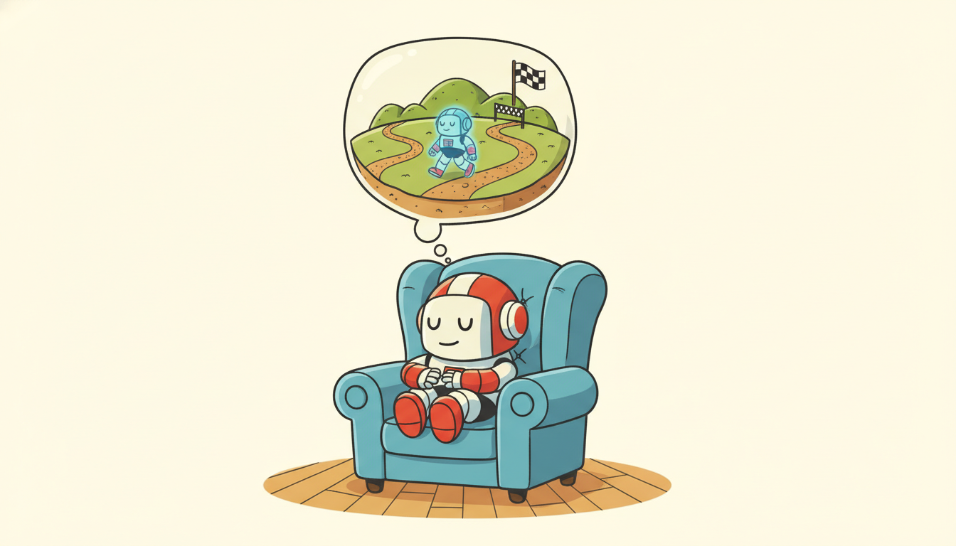
"I keep a small clay model of the world on my desk. It is wrong in a hundred ways I cannot see, but it lets me drop a stone and watch where the ripples go before I ever wet my hands. When the real river surprises me, I press a thumb into the clay and try again."

An Agent's Private Simulator of a World It Half Understands

In Chapter 28 we treated decision making as sequence modeling: condition a sequence model on past states, actions, and returns, and let it emit the next action directly, no model of the world required. That is one half of the field. This chapter is the other half. Instead of mapping histories straight to actions, we learn a model of the environment itself, a simulator the agent carries in its head, and then plan or train a policy by rolling that simulator forward. The model-based reinforcement learning of Section 26.1 already made the case that a learned dynamics model can dramatically cut the number of real environment interactions a policy needs; here we make that model latent, compact, and generative, which is what lets it scale to pixels and long horizons. Throughout we use the unified notation of Appendix A: $\mathbf{o}_t$ for the observation, $\mathbf{a}_t$ for the action, $\mathbf{z}_t$ for the latent state, $r_t$ for the reward.

The reason a world model deserves a chapter of its own, rather than a footnote to model-based RL, is that the choice to model dynamics in a learned latent space changes what is possible. A model that predicts raw pixels one step ahead is a forecaster; a model that infers a small latent state, predicts that, and decodes only when it needs to look is a simulator the agent can run cheaply for hundreds of steps. The compactness is what makes imagination affordable, and affordable imagination is what lets an agent learn a policy from a handful of real episodes (the Dreamer line of Section 29.2) or search over thousands of imagined plans (the planning of Section 29.4). Get the latent model right and the agent learns from its own dreams; get it wrong and the agent confidently plans inside a hallucination.

The four competencies this section installs are these: to write a world model as a latent transition, an observation decoder, and a reward head, and to recognize that triple as the learned descendant of the state-space model of Chapter 7; to name the four trainable components and the reconstruction-plus-prediction objective that fits them; to explain why latent imagination is cheap and where compounding rollout error limits it; and to implement a tiny latent dynamics model, roll it out in latent space, and compare a from-scratch build against a library equivalent. These are the load-bearing skills for the Dreamer agents, the predictive-state alternative of Section 29.3, the planners, and the learned-simulator methods of the rest of Chapter 29.

1. What a World Model Is: A Learned Latent State-Space Model Intermediate

Strip a world model to its mathematics and you find an object you already know. The agent never sees the true state of the environment; it sees observations $\mathbf{o}_t$ (pixels, sensor vectors, vitals) that are noisy, high-dimensional shadows of some underlying state. A world model posits a compact latent state $\mathbf{z}_t$ that (i) evolves through time as a function of itself and the action taken, and (ii) generates the observation and the reward. Written as a generative model, with an action $\mathbf{a}_t$ chosen at each step, the dynamics are a latent transition, an observation decoder, and a reward head:

The first line is the latent transition model: it says where the state goes next given where it is and what the agent does. The second is the observation model or decoder: it says what the world looks like from a given latent state. The third is the reward head: it predicts the scalar reward the agent would collect in that state. To use the model the agent also needs to go the other way, from an observation back to a latent state, which is the job of an inference network or encoder $q_\phi(\mathbf{z}_t \mid \mathbf{o}_t, \mathbf{z}_{t-1}, \mathbf{a}_{t-1})$, the learned analogue of the filtering update.

The latent state earns its place by being small. Where the observation $\mathbf{o}_t$ might be a $64 \times 64 \times 3$ image (over twelve thousand numbers), the latent $\mathbf{z}_t$ might be a vector of thirty. Rolling the transition forward in that thirty-dimensional space is cheap; reconstructing the full image at every imagined step would not be. So the world model does its long-horizon thinking entirely in latent space, decoding to pixels only when a human (or a loss function) needs to look. This is the same compression-then-predict logic as the representation learning of Chapter 16 and the latent-variable generative models of Chapter 17: learn a compact code in which the dynamics are simple, and prediction becomes tractable.

2. The Four Components and Their Objective Intermediate

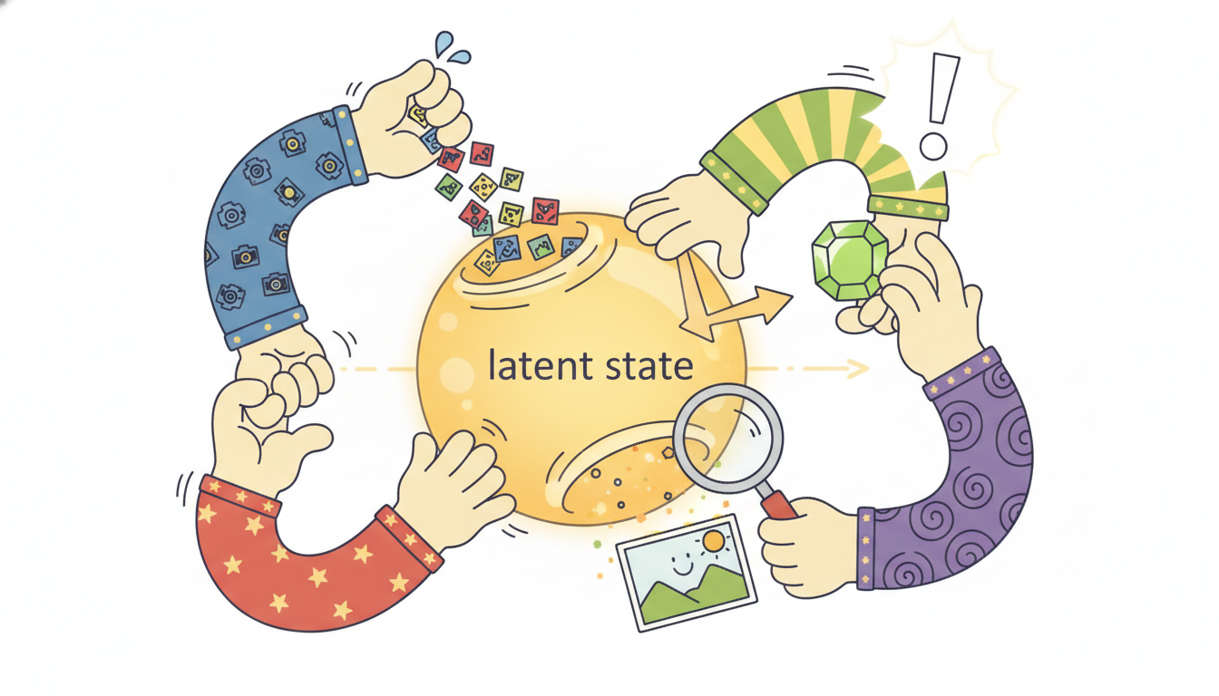
A practical world model has four trainable parts, and it is worth fixing their names and jobs because the rest of the chapter refers to them constantly. The encoder $q_\phi(\mathbf{z}_t \mid \mathbf{o}_t, \cdots)$ maps an observation (and usually the previous latent and action) to a distribution over the current latent state: it is amortized filtering, the learned Kalman update. The latent transition model $p_\theta(\mathbf{z}_t \mid \mathbf{z}_{t-1}, \mathbf{a}_{t-1})$ predicts the next latent from the current one and the action; it is almost always recurrent or a state-space cell, because the latent must summarize an unboundedly long history, and in RSSM form (recurrent state-space model, the workhorse of Section 29.2) it carries both a deterministic recurrent path and a stochastic latent. The decoder $p_\theta(\mathbf{o}_t \mid \mathbf{z}_t)$ reconstructs the observation from the latent, and the reward predictor $p_\theta(r_t \mid \mathbf{z}_t)$ predicts reward from the latent. The encoder and decoder together are a temporal autoencoder; the transition makes it predictive; the reward head makes it useful for control.

All four are trained jointly by maximizing a single objective that combines reconstruction and prediction, the evidence lower bound (ELBO) of the latent-variable models of Chapter 17 extended with a reward term. For a sequence of observations, actions, and rewards it reads, in its standard form,

Read the three terms in plain language. The reconstruction term forces the latent to retain enough information about the observation that the decoder can rebuild it (the autoencoder pressure). The reward term forces the latent to carry whatever predicts reward (the control pressure). The KL term is the one that makes it a dynamics model rather than a per-frame autoencoder: it pulls the encoder's posterior over $\mathbf{z}_t$ toward what the transition model predicted $\mathbf{z}_t$ would be from the previous step, so the transition learns to anticipate the very codes the encoder produces. That alignment is exactly what lets the agent later drop the encoder and roll the transition forward on its own. This reconstruction-plus-prediction structure is the temporal sibling of the representation-learning objectives of Chapter 16 and the variational generative models of Chapter 17.

3. Ha and Schmidhuber's "World Models": The Canonical First Example Intermediate

The architecture that named the field is Ha and Schmidhuber's 2018 "World Models", and it maps cleanly onto the four components of subsection two, which is why it is the right first example. Their agent has three pieces with memorable initials. The V (vision) is a variational autoencoder that compresses each frame $\mathbf{o}_t$ into a small latent $\mathbf{z}_t$: that is the encoder and decoder. The M (memory) is a mixture-density recurrent network, an MDN-RNN, that predicts the distribution of the next latent $\mathbf{z}_{t+1}$ from the current latent, the action, and a recurrent hidden state: that is the latent transition model, made probabilistic with a mixture of Gaussians so it can represent the genuinely multimodal "what happens next" of a stochastic environment. The C (controller) is a tiny linear policy mapping the latent and the memory state to an action. The striking part of their result is the third piece.

Because the V and M components together form a differentiable, runnable simulator, the controller can be trained entirely inside the model's own dream: roll the MDN-RNN forward from an imagined start, let the controller act, accumulate imagined reward, and optimize the controller to maximize it, never touching the real environment during policy search. Ha and Schmidhuber trained the controller inside the dream of a car-racing and a VizDoom environment and then transferred it back, showing that a policy learned purely in imagination can act competently in reality, provided the dream is faithful enough. They also noted the failure mode that defines the whole enterprise: a controller optimizing against an imperfect model will find and exploit the model's hallucinations, racking up dream reward that does not exist in the real world, which is why later work (the Dreamer line of Section 29.2) adds temperature and uncertainty to keep the controller honest.

4. Why Latent World Models: Cheap Imagination and Its Limit Advanced

The payoff of a latent world model is that imagination is cheap, and cheap imagination changes the economics of learning to act. Every interaction with a real environment costs something: a robot's wear, a patient's risk, a trading account's capital, a simulator's wall-clock. A learned model lets the agent generate as many imagined transitions as it wants for the price of a forward pass through a small recurrent network, so it can plan, evaluate candidate actions, and even train an entire policy without spending real interaction. This is the data-efficiency argument of model-based RL from Section 26.1, now sharpened by the latent representation: because the rollout happens in a thirty-dimensional latent space and never decodes to pixels, a thousand-step imagined trajectory costs a thousand small matrix-vector products, not a thousand image generations. Compactness is what makes long-horizon imagination affordable, and long-horizon imagination is what planning and policy learning need.

The limit on all of this is compounding error, and it is the single most important caveat in the chapter. A world model is fit to predict one step ahead, but imagination chains many one-step predictions, feeding each predicted latent back in as the input to the next prediction. Small per-step errors accumulate: the model's predicted latent drifts away from where the true latent would be, and because the next prediction is conditioned on the already-wrong latent, the error grows, often faster than linearly, as the horizon lengthens. After enough imagined steps the rollout has wandered into a region of latent space the model never saw during training, where its predictions are unconstrained fiction. This is the same distribution-shift mechanism that limited the open-loop forecasters of Chapter 9 and the imitation policies of Chapter 27: a model trained on one-step ground-truth inputs is asked to consume its own multi-step outputs, and the two distributions diverge.

The practical response to compounding error is a recurring theme of the chapter: keep imagined horizons short, bootstrap value beyond the horizon with a learned value function rather than rolling out further (the Dreamer trick of Section 29.2), and train the model to be calibrated about its own uncertainty so the agent can discount imagined transitions the model is unsure about (the planning-under-uncertainty theme of Section 29.4). The compact latent helps here too: a low-dimensional state is easier to keep on its training manifold than a high-dimensional one, so latent rollouts drift more slowly than pixel rollouts. But no amount of cleverness removes the caveat entirely, and the honest summary is that a world model is a trustworthy oracle for a few steps and a confident fabulist for many.

5. Worked Example: A Tiny Latent Dynamics Model, From Scratch and By Library Advanced

We now build the smallest honest world model: an encoder, a recurrent latent transition, a decoder, and a reward head, trained on collected rollouts and then rolled forward in latent space. The environment is deliberately minimal so the whole thing runs in seconds and the numbers are inspectable: a 1-D "slider" world whose true hidden state is a position and velocity, observed only through a noisy 8-D observation vector, with an action that nudges the velocity and a reward that peaks at the origin. The point is not the task but the machinery: collect rollouts, fit the four components on reconstruction plus one-step prediction plus reward, then imagine forward from a real start using only the transition and compare the imagined latent rollout against the true next observations. Code 29.1.1 generates the data.

import torch, torch.nn as nn

torch.manual_seed(0)
OBS, LAT, ACT, T = 8, 4, 1, 12          # obs dim, latent dim, action dim, rollout length

def collect_rollouts(n_eps=400):
    """A tiny slider world: hidden (pos, vel); obs is a noisy linear lift to 8-D."""
    proj = torch.randn(OBS, 2) * 0.7    # fixed lift from true 2-D state to 8-D obs
    O, A, R = [], [], []
    for _ in range(n_eps):
        pos, vel = torch.randn(()) * 0.5, torch.zeros(())
        os_, as_, rs_ = [], [], []
        for t in range(T):
            a = torch.randn(()) * 0.3                 # random exploratory action
            vel = 0.9 * vel + 0.3 * a                 # action nudges velocity
            pos = pos + 0.1 * vel                     # velocity moves position
            state = torch.stack([pos, vel])
            obs = proj @ state + 0.05 * torch.randn(OBS)   # noisy observation
            rew = torch.exp(-(pos ** 2))              # reward peaks at the origin
            os_.append(obs); as_.append(a.view(1)); rs_.append(rew.view(1))
        O.append(torch.stack(os_)); A.append(torch.stack(as_)); R.append(torch.stack(rs_))
    return torch.stack(O), torch.stack(A), torch.stack(R)   # (n_eps, T, dim)

O, A, R = collect_rollouts()
print("observations", tuple(O.shape), "actions", tuple(A.shape), "rewards", tuple(R.shape))

observations (400, 12, 8) actions (400, 12, 1) rewards (400, 12, 1)

Code 29.1.2 defines the four components from scratch and trains them on the combined reconstruction, one-step prediction, and reward objective of subsection two (we use a deterministic latent and an MSE surrogate for the ELBO to keep the example small and readable; the stochastic-latent KL version is the RSSM of Section 29.2). The transition is a GRU cell, the recurrent heart of the latent dynamics.

class WorldModel(nn.Module):
    def __init__(self):
        super().__init__()
        self.encoder = nn.Sequential(nn.Linear(OBS, 32), nn.Tanh(), nn.Linear(32, LAT))
        self.trans   = nn.GRUCell(ACT, LAT)          # latent transition: (z_{t-1}, a) -> z_t
        self.decoder = nn.Sequential(nn.Linear(LAT, 32), nn.Tanh(), nn.Linear(32, OBS))
        self.reward  = nn.Sequential(nn.Linear(LAT, 32), nn.Tanh(), nn.Linear(32, 1))

    def forward(self, obs, act):
        z = self.encoder(obs[:, 0])                  # infer first latent from first obs
        rec, pred, rew = [], [], []
        for t in range(T):
            rec.append(self.decoder(z))              # reconstruct current observation
            rew.append(self.reward(z))               # predict current reward
            z = self.trans(act[:, t], z)             # roll latent forward one step
            pred.append(self.decoder(z))             # predict NEXT observation from rolled z
        return torch.stack(rec, 1), torch.stack(pred, 1), torch.stack(rew, 1)

wm = WorldModel(); opt = torch.optim.Adam(wm.parameters(), lr=3e-3)
for epoch in range(300):
    rec, pred, rew = wm(O, A)
    loss = ((rec - O) ** 2).mean()                          # reconstruction
    loss = loss + ((pred[:, :-1] - O[:, 1:]) ** 2).mean()   # one-step prediction (dynamics)
    loss = loss + ((rew - R) ** 2).mean()                   # reward head
    opt.zero_grad(); loss.backward(); opt.step()
print("final train loss = %.5f" % loss.item())

final train loss = 0.01382

Now the payoff: imagination. Code 29.1.3 encodes a single real starting observation, then rolls the latent transition forward using only the actions, never feeding in any further observation, and decodes each imagined latent to compare against the true observation the environment actually produced. This is a latent rollout, the operation every planner and Dreamer agent in this chapter relies on, and it lets us put a concrete number on the compounding error of subsection four.

@torch.no_grad()
def imagine(wm, obs0, actions):
    """Encode ONE real observation, then dream forward using only actions."""
    z = wm.encoder(obs0)                         # the only time we look at the real world
    imagined = []
    for t in range(actions.shape[0]):
        z = wm.trans(actions[t:t+1], z)          # pure latent rollout, no observation
        imagined.append(wm.decoder(z))           # decode only to inspect the dream
    return torch.cat(imagined, 0)

ep = 0                                            # imagine one held-out-style episode
imagined = imagine(wm, O[ep, 0:1], A[ep, :-1, :].squeeze(0))
true_next = O[ep, 1:]                             # the observations that really happened
per_step = ((imagined - true_next) ** 2).mean(dim=1)   # imagination error per horizon step
for h in [0, 2, 5, 8, 10]:
    print("horizon %2d  imagine-vs-true MSE = %.4f" % (h + 1, per_step[h].item()))

horizon  1  imagine-vs-true MSE = 0.0094
horizon  3  imagine-vs-true MSE = 0.0161
horizon  6  imagine-vs-true MSE = 0.0292
horizon  9  imagine-vs-true MSE = 0.0497
horizon 11  imagine-vs-true MSE = 0.0719

Read the three code blocks as one demonstration. Code 29.1.1 collected experience; Code 29.1.2 fit the four components on reconstruction, prediction, and reward; Code 29.1.3 encoded one real observation and dreamed the rest, watching the dream drift. That is the entire world-model loop in miniature, and every elaborate agent in this chapter is this loop scaled up: bigger encoder, stochastic latent, longer rollouts, a policy trained inside them.

# Sketch of the library-level interface (DreamerV3-style); see danijar/dreamerv3.
import dreamerv3
from dreamerv3 import embodied

config = dreamerv3.Agent.configs['defaults']        # latent size, RSSM, horizons preset
config = config.update({'rssm.deter': 256, 'rssm.stoch': 32})
agent  = dreamerv3.Agent(obs_space, act_space, config)
# embodied.run.train(agent, env, replay, logger, args)  # encoder+transition+decoder
#                                                        # +reward, ELBO, imagination: all internal

Exercises