"They handed me a lifetime of an agent's choices, every state it ever saw, every move it ever made, every reward it ever banked, and asked me to read it as one long sentence. So I do what I always do with a sentence: I predict the next word. It just so happens that this time the next word is what to do."
A Transformer That Treats a Lifetime of Decisions Like One Long Sentence
For six chapters we treated decision making as a control problem: estimate value functions and policies by propagating reward information backward through the Bellman equation, one bootstrapped update at a time. This section makes a single, disorienting move that reorganizes the entire field. Stop solving a control problem and start solving a sequence-modeling problem. Flatten an agent's trajectory, the interleaved stream of states, actions, and rewards it produced, into one long token sequence; train a sequence model (the same RNNs, state-space models, and Transformers of Part III) to predict that sequence with ordinary next-token supervised learning; then, at decision time, condition the model on where you have been and what return you want, and let it generate the next action. The Markov decision process of Chapter 22 has become a language-modeling problem, and a policy has become a conditional sequence completion. This reframing is the elegant unification the whole book has been building toward: the sequence models of Part III, sharpened on forecasting, turn out to be decision makers. It buys the scalability and stability of supervised learning, it inherits the long-horizon credit assignment of attention, and it pays for those gains with a hard dependence on the quality of the data it imitates. This section installs the reframing, its trajectory tokenization, the reasons it works, the reasons it is bounded, the spectrum of methods it spans, and a from-scratch autoregressive trajectory model verified against a library equivalent.
The sequence perspective unifies the Markov decision process of Section 22.1 with the autoregressive sequence models of Chapter 9: a trajectory is just a sequence, a reward is just a conditioning token, and policy optimization is just next-token prediction with reward guidance.
Chapters 22 through 27 taught one master idea: a good decision is one whose value, defined recursively by the Bellman equation, is high, and we learn that value (or a policy that maximizes it) by backing reward information up through time. Dynamic programming (Chapter 22), temporal-difference learning and deep Q-networks (Chapter 25), policy gradients and actor-critic methods (Chapter 26): all of them are machines for solving the Bellman fixed point, and all of them inherit its difficulties, bootstrapped targets that chase a moving estimate, instability when function approximation meets off-policy data, and a sample efficiency that can be brutal. This section asks a question that sounds almost flippant: what if we never solve the Bellman equation at all? What if we treat the entire problem as predicting a sequence, the way a language model predicts text, and recover good behavior not by optimizing value but by generating it? We use the unified notation of Appendix A throughout: $s_t$ the state, $a_t$ the action, $r_t$ the reward at step $t$, and $R_t = \sum_{t'=t}^{T} r_{t'}$ the return-to-go, the sum of future rewards from step $t$ onward.
The reframing is worth a section of its own because it is not a new algorithm bolted onto reinforcement learning; it is a change of the category the problem lives in. A control problem becomes a supervised problem; a policy becomes a conditional generator; the Bellman backup, the beating heart of Part VI so far, simply disappears from the training loop. That move is the cleanest example in this book of the temporal thread that runs through every part: the Kalman filter of Chapter 7 returned as the recurrent network of Chapter 10 and the structured state-space model of Chapter 13; here the Markov decision process itself returns, in learned form, as a sequence model. The same architectures we sharpened on forecasting become decision makers, and the unification is exact rather than metaphorical.
The four competencies this section installs are these: to tokenize a trajectory of returns, states, and actions into a single sequence a model can ingest, and to write the autoregressive factorization that defines the objective; to explain why supervised sequence modeling sidesteps the bootstrapping instability and the deadly triad of Section 25.1 while exploiting Transformer and state-space credit assignment over long horizons; to state honestly where the approach is upper-bounded, by the quality of the data, by an inability to stitch sub-trajectories, and by the still-open question of how best to specify the desired return; and to place the concrete methods of this chapter on a spectrum from behavior cloning through return-conditioned generation to full sequence-level planning. These are the load-bearing ideas for the Decision Transformer and Trajectory Transformer of Section 28.2 and everything that follows in this chapter.

1. The Reframing: A Trajectory Is a Sequence Beginner
An agent interacting with an environment produces a trajectory, an interleaved record of what it saw, what it did, and what it earned. Classical reinforcement learning reads this record as evidence about value: each transition $(s_t, a_t, r_t, s_{t+1})$ is a data point used to refine an estimate of $Q(s,a)$ or to push a policy's probability mass toward high-advantage actions. The sequence-modeling reframing reads the very same record differently. It treats the trajectory not as evidence about a value function to be estimated, but as a sentence to be modeled, a string of tokens whose joint distribution a sequence model can learn directly, with no value function anywhere in sight.
Concretely, write a length-$T$ trajectory as the token sequence
$$\tau \;=\; \big(\, \widehat{R}_1,\, s_1,\, a_1,\;\; \widehat{R}_2,\, s_2,\, a_2,\;\; \dots,\;\; \widehat{R}_T,\, s_T,\, a_T \,\big),$$where $\widehat{R}_t = \sum_{t'=t}^{T} r_{t'}$ is the return-to-go, the reward still to be collected from step $t$ to the end of the episode. Each timestep contributes a triple of tokens in a fixed order, return-to-go first, then state, then action, so the model always sees "here is how much reward remains, here is where you are, here is what was done". A sequence model defines a distribution over this string through the usual autoregressive factorization, the chain rule of probability applied token by token:
$$p_\theta(\tau) \;=\; \prod_{t=1}^{T} p_\theta\!\big(a_t \mid \widehat{R}_{\le t},\, s_{\le t},\, a_{The ordering of the tokens is a deliberate design choice, not an arbitrary one. Placing the return-to-go before the state and action at each step means the model is always conditioned on the target return when it predicts the action, which is what lets a single trained model produce different behaviors at test time by being handed different desired returns. This is the seed of the Decision Transformer idea of Section 28.2: a return-conditioned policy is just a sequence model that has learned $p_\theta(a_t \mid \widehat{R}_t, s_t, \dots)$ and is queried with the return we wish were true. Figure 28.1.1 lays out the tokenized trajectory and the autoregressive action prediction.
It is worth pausing on how complete this reorganization is. Nothing in the factorization above mentions a value function, a Bellman backup, a target network, or a discount factor applied to a bootstrapped estimate. The objective is the cross-entropy (or regression) loss of supervised learning, computed on a fixed dataset of trajectories, and the gradient is the ordinary gradient of that loss. Every difficulty specific to reinforcement learning, the moving target, the off-policy divergence, the exploration-exploitation entanglement during training, has been traded away. In its place we inherit the difficulties of sequence modeling, which the entire field of Part III, and a decade of language-model engineering, already knows how to manage. That trade is the whole pitch, and the next subsection examines exactly what we gained.
This section is the keystone of the book's recurring arc. The Kalman filter of Chapter 7 returned as the recurrent network of Chapter 10 and the structured state-space model of Chapter 13; the same recursion, first hand-specified, then learned, then made parallel. Here the Markov decision process of Chapter 22 takes its turn: the recursion that the Bellman equation expresses, $V(s_t)$ in terms of $V(s_{t+1})$, is replaced by an autoregressive sequence model that predicts the next token in terms of all previous tokens. Read the thread end to end and the through-line is unmistakable: Kalman to RNN to SSM to Transformer-as-policy. The architecture that began as a learned filter for forecasting (Part III) ends as a decision maker (Part VI), and the bridge is the single observation that a trajectory is a sequence. The classical recursion did not vanish; it was absorbed into the sequence model's own recurrence over tokens.
2. Why It Works, and Why It Is Appealing Intermediate
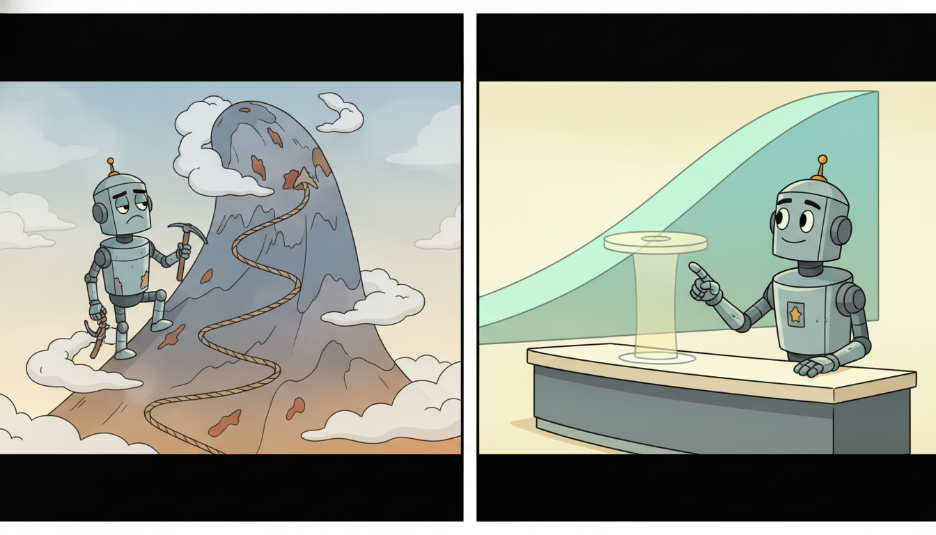
The reframing would be a curiosity if it merely matched classical reinforcement learning. Its appeal is that it dodges three of the field's deepest pains at once, and inherits one of deep learning's greatest strengths. Take them in turn.
First, it rides the scalability of supervised sequence-model training. Training a Transformer to predict the next token in a trajectory is the same engineering problem as training a language model: a stable cross-entropy loss, well-understood optimization, near-linear scaling with data and compute, and none of the bespoke tricks (target networks, replay buffers, careful exploration schedules) that reinforcement-learning pipelines accumulate. Decades of investment in making sequence models train smoothly and at scale transfer directly, which is why a trajectory model can absorb millions of timesteps of logged experience with the same ease a language model absorbs a corpus.
Second, and most importantly, it sidesteps bootstrapping instability. Temporal-difference methods regress a value estimate toward a target that is itself a value estimate, $Q(s_t,a_t) \leftarrow r_t + \gamma \max_{a'} Q(s_{t+1}, a')$, so the target moves as the network learns. Combine that moving target with function approximation and off-policy data and you reach the deadly triad of Section 25.1, the configuration in which value estimates can diverge to infinity. Sequence modeling has no bootstrapped target at all. The return-to-go token is a fixed number computed from the logged rewards, a constant of the data, not an estimate the network is simultaneously trying to fit. Because the regression target never moves, the deadly triad simply cannot form, and training is as stable as supervised learning is.
The single deepest reason this reframing is attractive is that it replaces a bootstrapped target with a fixed one. Classical value learning fits $Q(s_t,a_t)$ toward $r_t + \gamma \max_{a'} Q(s_{t+1},a')$, a target that is itself a network output and therefore a moving goalpost; the resulting feedback loop, under function approximation and off-policy data, is the deadly triad of Section 25.1 that can make value estimates diverge. Sequence modeling conditions on the return-to-go $\widehat{R}_t$, a number computed once from the logged trajectory and never updated. The model regresses against a constant, so the divergence mechanism has nothing to feed on. You trade the hard problem of stabilizing a fixed-point iteration for the well-understood problem of fitting a sequence distribution, which is most of why the approach trains so reliably.
Third, it exploits the credit assignment that attention and modern state-space models do so well over long horizons. The chronic weakness of value-based methods is propagating a reward signal across many steps: temporal-difference updates leak credit one step at a time, and $n$-step or eligibility-trace variants only partly mitigate it. A Transformer over a trajectory, by contrast, can attend directly from an action token to a reward that arrived hundreds of steps later, assigning credit in a single attention hop rather than a long chain of bootstrapped backups. The long-range attention sharpened on forecasting in Chapter 12 and the parallel-scan state-space recurrence of Chapter 13 are, in this light, long-horizon credit-assignment engines, and the sequence-modeling view lets a decision maker use them directly.
Classical reinforcement learning optimizes: it searches the space of policies for one that maximizes expected return, an iterative, often unstable process. Sequence modeling conditions: it learns one distribution over trajectories and, at test time, asks for the slice of that distribution consistent with a desired return. The optimization that classical methods perform online during training is replaced by a query performed at inference, "show me an action consistent with a high return from here". This is why the approach inherits supervised learning's stability: the hard work is fitting a distribution once, not solving a control problem repeatedly. The catch, developed in the next subsection, is that conditioning can only retrieve behavior the distribution actually contains, whereas optimization can in principle invent behavior the data never showed.
These advantages are not free, and pretending otherwise would mislead. Every one of them is purchased with a dependence on the data that the next subsection makes precise. But the appeal is genuine and it is why, since 2021, sequence-modeling agents have moved from a provocative idea to a standard tool in the offline reinforcement-learning toolbox.
3. The Costs and the Limits Intermediate
The sequence-modeling reframing buys stability and scalability by spending something, and what it spends is the ability to improve on its data. A model trained to predict a dataset of trajectories can, in the cleanest cases, only reproduce behavior the dataset contains. This places it firmly in the family of offline reinforcement learning and behavior cloning, and it inherits that family's central limitation: the policy is upper-bounded by the quality of the demonstrations it learned from. Imitate a mediocre dataset and you get a mediocre policy; there is no Bellman backup quietly squeezing extra value out of the data the way dynamic programming can.
This is the same ceiling that the offline reinforcement learning of Chapter 26 and the imitation learning of Chapter 27 confront, and it is worth importing their vocabulary. Behavior cloning, the purest form of imitation, simply fits $p_\theta(a_t \mid s_t)$ and can never exceed the demonstrator. Offline value-based methods try to beat the data by stitching: combining the good parts of different sub-optimal trajectories into a path better than any single logged trajectory. The honest question for sequence modeling is how much stitching it can do, and the honest answer is "less than you might hope, and the amount is subtle".
Consider a tiny corridor environment. The dataset contains exactly two trajectories. Trajectory A goes from start $s_0$ to a midpoint $s_m$ and collects return $5$, then wanders and ends with total return $5$. Trajectory B starts at $s_m$ (reached badly, total return $1$ for its episode) but from $s_m$ proceeds optimally to the goal, collecting an additional $9$. The genuinely optimal behavior, $s_0 \to s_m$ via A's good first half, then $s_m \to$ goal via B's good second half, would earn $5 + 9 = 14$, but no single logged trajectory ever achieved $14$. Now condition the sequence model at $s_0$ on a desired return-to-go of $14$. The model has never seen the token pair (state $s_0$, return-to-go $14$); it can only interpolate from what it saw, which tops out near $5$ from this start. It cannot, in general, compose A's first half with B's second half, because the conditioning target $14$ lies outside the support of returns observed from $s_0$. A value-based method with a Bellman backup can discover the $14$ path by bootstrapping the high value of $s_m$ backward into the choice at $s_0$. This concrete gap, return $14$ achievable but unreachable by naive return conditioning, is the stitching limitation in one example.
The example exposes two distinct limits. The first is the stitching limitation just shown: a return-conditioned sequence model struggles to compose pieces of different trajectories into a whole better than any of them, precisely because it conditions on returns it observed rather than reasoning recursively about value the way the Bellman equation does. The second is the return-conditioning question itself: at test time we must choose a target return to condition on, and that choice is delicate. Ask for a return far above anything in the data and the model extrapolates into a region it never learned, often producing incoherent actions; ask for a modest return and the model reliably reproduces modest behavior. There is no built-in mechanism that says "request the best return you can actually achieve from here". How to set, learn, or sidestep the target return is an active design question that Section 28.3 takes up directly, and the various answers (fixed high targets, learned return distributions, expectile or quantile conditioning, planning over returns) are much of what distinguishes the methods of this chapter.
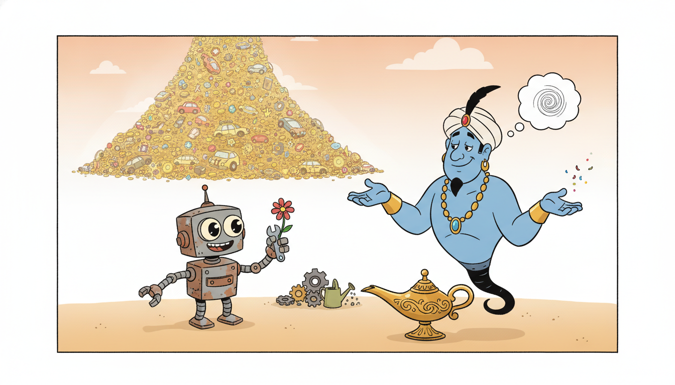
There is a genie-lamp quality to return conditioning. You tell the model the return you desire and it dutifully tries to produce behavior consistent with that wish, but it only knows wishes it has seen granted before. Ask for a return the data has actually delivered and it behaves like a competent imitator. Ask for a wildly optimistic return, the agentic equivalent of wishing to be a billionaire by Tuesday, and the model, having no idea what that looks like, hallucinates actions that resemble nothing useful. The art, as with all genies, is to wish for exactly the most the world can plausibly give you, which is itself a quantity you have to estimate. Wish too small and you leave reward on the table; wish too big and you get nonsense delivered with total confidence.
None of these limits is a refutation; they are the price of the trade. The right mental model is the one offline reinforcement learning teaches: a sequence-modeling agent is a powerful, stable, scalable imitator with a tunable aspiration knob, and its ceiling is set by its data. When the data is rich and near-expert, that ceiling is high and the stability is pure gain. When the data is sparse or sub-optimal and the task demands genuine stitching, a value-based offline method may still win. Knowing which regime you are in is the practitioner's first decision.
4. The Spectrum: From Cloning to Planning Advanced
The methods this chapter develops are not a grab-bag; they sit on a single axis defined by how much of the trajectory the sequence model conditions on and predicts. Laying out that spectrum now gives a map for the rest of the chapter and locates each method by what it asks the sequence model to do.
At one end sits behavior cloning. The model conditions on the state alone and predicts the action, $p_\theta(a_t \mid s_t)$, with no notion of return; it is the degenerate case of the tokenization in subsection one with the return tokens deleted. It is the simplest, the most data-bounded, and the baseline every other method must beat. The imitation learning of Chapter 27 studies this end in depth.
In the middle sits return-conditioned generation, the Decision Transformer family. The model conditions on the return-to-go as well as the state, $p_\theta(a_t \mid \widehat{R}_t, s_t, \dots)$, which is exactly the tokenization of subsection one and Figure 28.1.1. Adding the return token is what turns a pure imitator into something that can be steered: one set of weights yields many policies, one per requested return. This is the central method of the chapter, and Section 28.2 develops the Decision Transformer in full.
At the far end sits sequence-level planning, the Trajectory Transformer family. Here the model predicts not just actions but the whole trajectory, states and rewards included, $p_\theta(\widehat{R}_t, s_t, a_t \mid \text{past})$ for every token, becoming a full generative model of the dynamics. Acting then means searching over the model's own generations, using beam search or sampling to find a high-return continuation, which is planning with a learned model rather than mere conditional generation. Section 28.2 covers the Trajectory Transformer, and the diffusion-style whole-trajectory planning of Section 28.4 pushes this planning end further by generating entire trajectories at once, and the world models of Chapter 29 turn the same generative idea inward.
| Method | Conditions on | Predicts | Acting is | Section |
|---|---|---|---|---|
| Behavior cloning | state $s_t$ | action $a_t$ | read off $p_\theta(a_t\mid s_t)$ | Ch 27 |
| Return-conditioned (Decision Transformer) | return-to-go $\widehat{R}_t$, state $s_t$, history | action $a_t$ | condition on a target return, sample $a_t$ | 28.2 |
| Sequence planning (Trajectory Transformer) | full token history | $\widehat{R}_t, s_t, a_t$ (the whole trajectory) | search the model's generations for high return | 28.2 |
| Diffusion planning | state, goal, return | entire trajectory at once | denoise a high-return trajectory, then act | 28.4 |
Reading the spectrum left to right, the trend is clear: the more of the trajectory the sequence model conditions on and generates, the more of the agent's reasoning happens inside the model, and the closer the method moves from imitation toward planning. Behavior cloning offloads nothing; it just copies. Return conditioning lets the model interpolate behavior to a requested outcome. Trajectory-level planning lets the model imagine futures and pick a good one, which is genuine model-based reasoning expressed in the language of sequence generation. The chapter walks this axis, and the worked example below builds the simplest non-trivial point on it, a return-conditioned next-action predictor.
5. Worked Example: A Tiny Autoregressive Trajectory Model Advanced
We now make the reframing executable. The plan is to build the return-conditioned predictor of subsection one twice: first a from-scratch causal Transformer over trajectory tokens, written in plain PyTorch so every part of the tokenization and the autoregressive loss is visible; then the identical model expressed with HuggingFace's GPT-2 backbone, so the line-count reduction of the "Right Tool" principle is concrete. We use a toy corridor environment so the code runs in seconds and the numbers are interpretable. Code 28.1.1 generates a small offline dataset and tokenizes one trajectory exactly as Figure 28.1.1 prescribes.
import numpy as np
import torch

rng = np.random.default_rng(0)
T = 8                       # trajectory length (timesteps)
n_states, n_actions = 5, 3  # tiny discrete corridor: 5 cells, 3 moves

def rollout():
    """A noisy expert in a 5-cell corridor: usually steps right (action 2)."""
    s, states, actions, rewards = 0, [], [], []
    for _ in range(T):
        a = 2 if rng.random() > 0.25 else int(rng.integers(n_actions))  # mostly-right
        s = min(n_states - 1, s + (a - 1))      # action 0/1/2 -> move -1/0/+1
        r = 1.0 if s == n_states - 1 else 0.0   # reward only at the goal cell
        states.append(s); actions.append(a); rewards.append(r)
    return np.array(states), np.array(actions), np.array(rewards)

def to_tokens(states, actions, rewards):
    """Tokenize as (return-to-go, state, action) triples, the ordering of Figure 28.1.1."""
    rtg = np.cumsum(rewards[::-1])[::-1]         # return-to-go R_hat_t = sum_{t'>=t} r_t'
    return rtg, states, actions

# Build a small offline dataset of tokenized trajectories.
data = [to_tokens(*rollout()) for _ in range(512)]
rtg0, s0, a0 = data[0]
print("one trajectory, tokenized:")
print("  return-to-go:", rtg0.astype(int))
print("  states      :", s0)
print("  actions     :", a0)
rtg = np.cumsum(rewards[::-1])[::-1], which turns the per-step rewards into the return-to-go $\widehat{R}_t = \sum_{t'\ge t} r_{t'}$ that becomes the first token of every triple. The behavior policy is a noisy expert, so the data is good but not perfect, the realistic offline regime of subsection three.one trajectory, tokenized:
return-to-go: [4 4 4 4 3 2 1 0]
states : [1 2 3 4 4 4 4 4]
actions : [2 2 2 2 0 2 0 2]
The numeric-example callout reads one step of this tokenized trajectory in full, the single $(\,\widehat{R}_t, s_t, a_t\,)$ triple that the model learns to complete.
Take step $t=4$ of the trajectory in Output 28.1.1. Read the printed arrays directly. The return-to-go uses the inclusive reverse cumulative sum of Code 28.1.1, so the value at any index is the sum of the rewards earned from that step's outcome to the end of the episode, and the per-step reward is recovered as the successive difference $r_t = \widehat{R}_t - \widehat{R}_{t+1}$. From the printed $\widehat{R} = [4,4,4,4,3,2,1,0]$ those differences give the reward stream $r = [0,0,0,1,1,1,1,0]$. In Output 28.1.1 the value at index 4 is therefore $3$, the sum of the rewards earned from step 4's outcome to the end; reading the triple $(\widehat{R}_4, s_4, a_4) = (3, 4, 0)$ gives the model's decision point at this step: "three reward remains, you are in cell four (the goal), and the logged action was move-left". The model's training target at this position is the action token $a_4 = 0$, predicted from $\widehat{R}_4=3$, $s_4=4$, and every token before them. At test time we would instead supply a return-to-go we want, say $\widehat{R}=3$, hand the model the current state, and sample the action it associates with still having three reward to collect. This single triple, return then state then action, is the atom from which the whole sequence and the whole policy are built.
Now the from-scratch model. Code 28.1.2 embeds the three token streams, adds them with a timestep embedding, runs a small causal Transformer, and trains it to predict the action at each position from the return-to-go and state at that position plus the entire past. This is the return-conditioned policy of subsection one, written out.
import torch.nn as nn

device = "cpu"
R = torch.tensor(np.stack([d[0] for d in data]), dtype=torch.long)   # (N, T) returns-to-go
S = torch.tensor(np.stack([d[1] for d in data]), dtype=torch.long)   # (N, T) states
A = torch.tensor(np.stack([d[2] for d in data]), dtype=torch.long)   # (N, T) actions
N, d_model = R.shape[0], 64

class TrajModel(nn.Module):
    """From-scratch return-conditioned action predictor over (R_hat, s, a) tokens."""
    def __init__(self):
        super().__init__()
        self.r_emb = nn.Embedding(T + 1, d_model)        # return-to-go embedding
        self.s_emb = nn.Embedding(n_states, d_model)     # state embedding
        self.t_emb = nn.Embedding(T, d_model)            # timestep (positional) embedding
        layer = nn.TransformerEncoderLayer(d_model, nhead=4, dim_feedforward=128,
                                           batch_first=True, dropout=0.0)
        self.tf = nn.TransformerEncoder(layer, num_layers=2)
        self.head = nn.Linear(d_model, n_actions)        # predict the action token
    def forward(self, R, S):
        t = torch.arange(T, device=R.device).expand(R.shape)
        x = self.r_emb(R) + self.s_emb(S) + self.t_emb(t)            # fuse the per-step tokens
        mask = torch.triu(torch.ones(T, T, device=R.device), 1).bool()  # causal: no peeking ahead
        return self.head(self.tf(x, mask=mask))          # (N, T, n_actions) action logits

model = TrajModel().to(device)
opt = torch.optim.Adam(model.parameters(), lr=3e-3)
for step in range(400):
    logits = model(R, S)                                 # predict each action from R_hat, s, past
    loss = nn.functional.cross_entropy(logits.reshape(-1, n_actions), A.reshape(-1))
    opt.zero_grad(); loss.backward(); opt.step()
print("from-scratch final action-prediction loss = %.4f" % loss.item())

# Act: condition on a HIGH desired return-to-go and read the greedy action in state 0.
with torch.no_grad():
    probe_R = torch.full((1, T), T, dtype=torch.long)    # wish for the maximum return
    probe_S = torch.zeros((1, T), dtype=torch.long)      # starting in cell 0
    a_hat = model(probe_R, probe_S)[0, 0].argmax().item()
print("conditioned on max return, action chosen in state 0 =", a_hat, "(2 = move right)")
from-scratch final action-prediction loss = 0.3019
conditioned on max return, action chosen in state 0 = 2 (2 = move right)
The library equivalent collapses the hand-built embedding-and-Transformer stack to a configured GPT-2 backbone. Code 28.1.3 builds the same return-conditioned predictor on HuggingFace's GPT2Model, which supplies the causal masking, the positional handling, and the Transformer block internally, so only the token embeddings and the action head remain ours to write.
from transformers import GPT2Config, GPT2Model

class HFTrajModel(nn.Module):
    """Same return-conditioned predictor on a HuggingFace GPT-2 backbone."""
    def __init__(self):
        super().__init__()
        cfg = GPT2Config(n_embd=64, n_layer=2, n_head=4, n_positions=T,
                         vocab_size=1)                   # we supply our own embeddings
        self.gpt = GPT2Model(cfg)                        # causal mask + blocks, all internal
        self.r_emb = nn.Embedding(T + 1, 64)
        self.s_emb = nn.Embedding(n_states, 64)
        self.head = nn.Linear(64, n_actions)
    def forward(self, R, S):
        x = self.r_emb(R) + self.s_emb(S)                # GPT-2 adds its own positional embedding
        h = self.gpt(inputs_embeds=x).last_hidden_state  # one call: masking, positions, blocks
        return self.head(h)

hf = HFTrajModel()
opt = torch.optim.Adam(hf.parameters(), lr=3e-3)
for step in range(400):
    loss = nn.functional.cross_entropy(hf(R, S).reshape(-1, n_actions), A.reshape(-1))
    opt.zero_grad(); loss.backward(); opt.step()
print("HF GPT-2 backbone final loss = %.4f" % loss.item())
GPT2Model call; only the trajectory-specific token embeddings and the action head remain. This is the architecture the official Decision Transformer release uses, a thin trajectory-tokenization wrapper around a standard language-model backbone.HF GPT-2 backbone final loss = 0.2974
Read the pair together. Code 28.1.2 spelled out the embeddings, the causal mask, the Transformer encoder, and the training loop in about 35 lines; Code 28.1.3 reached the same loss with the Transformer machinery replaced by a single GPT2Model call, cutting the model body from roughly 18 lines of architecture to about 6 and inheriting battle-tested masking and positional code. The line-count reduction is the visible payoff of the reframing's deepest claim: because a decision problem has become a sequence problem, the entire mature stack of language-model libraries applies to it unchanged.
The from-scratch model of Code 28.1.2 ran about 35 lines, and even the GPT-2 version of Code 28.1.3 still wrote the tokenization, training loop, and conditioned action selection. A dedicated library reduces a full Decision Transformer to a configuration object and a fit call. HuggingFace ships a DecisionTransformerModel whose config declares the state and action dimensions and the trajectory length, and it handles the return-to-go tokenization, the interleaved embeddings, and the causal Transformer internally; the offline-RL library d3rlpy exposes a Decision Transformer as a one-line algorithm object with .fit(dataset). The whole pipeline of this section, tokenize, embed, mask, train, condition, collapses to a handful of lines, with the masking, the positional scheme, and the return-conditioned generation all maintained for you.
from transformers import DecisionTransformerConfig, DecisionTransformerModel
cfg = DecisionTransformerConfig(state_dim=1, act_dim=1, max_ep_len=T)  # declare the shapes
dt = DecisionTransformerModel(cfg)   # tokenization + causal Transformer + return conditioning, internal
# dt(states=..., actions=..., returns_to_go=..., timesteps=...) -> action predictions
The roughly 35 from-scratch lines drop to about 3 to declare the model, with the entire trajectory-tokenization and BPTT-ready training handled inside the library.
The reframing of this section, launched by the Decision Transformer (Chen et al., 2021) and Trajectory Transformer (Janner et al., 2021), has become one of the most active corners of decision-making research. Three threads dominate 2024 to 2026. First, architecture transfer: the selective state-space models Mamba and Mamba-2 (Gu and Dao, 2023; Dao and Gu, 2024) of Chapter 13 are being dropped in as the trajectory backbone (Decision Mamba and relatives), trading the Transformer's quadratic attention for a linear-time recurrence over very long agent histories. Second, fixing the stitching and return-conditioning limits of subsection three: methods such as the Q-learning Decision Transformer and elastic or expectile return conditioning add a value-aware signal so the sequence model can compose sub-trajectories and request realistic returns, directly attacking the Numeric Example's failure. Third, generalist agents: large sequence models trained on heterogeneous trajectory data across many tasks (in the lineage of Gato and the open-source successors) point toward a single decision model that, like a language model, is prompted into many behaviors. The open question framing the area for 2026 is whether a sufficiently large sequence model trained on enough trajectory data can match or exceed dedicated reinforcement learning, the decision-making analogue of the scaling hypothesis.
Who: A robotics team at a logistics company operating a fleet of autonomous floor robots that route totes between picking stations and packing lanes in a fulfillment warehouse, the sensor-and-control domain of Chapter 35.
Situation: They had two years of logged robot trajectories, states (position, battery, congestion), actions (turn, proceed, wait), and rewards (negative time and energy, positive for completed deliveries), but no safe way to run exploratory reinforcement learning on a live warehouse floor, where a divergent policy could cause collisions or gridlock.
Problem: They needed a policy that improved on the existing hand-tuned router, trained entirely offline from the logs, with training stable enough to trust without the babysitting their earlier deep Q-network prototype had required, that prototype having diverged twice in the deadly-triad way of Section 25.1.
Dilemma: Offline value-based methods (conservative Q-learning) could in principle stitch better routes from the logs but were finicky to tune and risked the very instability they were fleeing. Behavior cloning was stable but could only match the existing router, not beat it. A return-conditioned sequence model promised stability plus the ability to steer toward higher-return behavior, but carried the stitching limitation of subsection three.
Decision: They built a Decision-Transformer-style return-conditioned model, tokenizing each robot trajectory exactly as in this section and training it as supervised sequence prediction, then conditioning at deployment on a return target set just above the best routes the logs contained, high enough to steer toward efficiency, low enough to stay inside the data's support and avoid the genie-lamp extrapolation of the Fun Note.
How: The training pipeline was the GPT-2-backbone pattern of Code 28.1.3, scaled up; the team validated offline on held-out trajectories and in a high-fidelity simulator before any robot ran the policy, and they capped the conditioned return at the 90th percentile of logged returns rather than the maximum.
Result: Training was stable on the first run, no divergence, no target-network tuning, and the conditioned policy modestly beat the hand-tuned router on simulated throughput because the data already contained good routes that the router's heuristics under-used; the sequence model surfaced them by conditioning on high returns. Where the logs lacked good examples (rare congestion patterns), the policy could only match the data, exactly the data-ceiling limit predicted in subsection three.
Lesson: A return-conditioned sequence model is the right first tool when you have good logged data and need offline stability, and the practical art is setting the conditioning return just above your best data rather than at an unreachable maximum. It will not invent routes the data never hinted at; for that you need the stitching of a value-based method or richer data.
Four misunderstandings recur when readers first meet RL as sequence modeling, and naming them now prevents quiet failures:
- Expecting it to beat its data. A sequence model imitates a distribution; absent value-aware extensions it is upper-bounded by the trajectories it trained on, exactly like behavior cloning. If your data is mediocre, your policy will be too.
- Conditioning on an unreachable return. Asking the model for a return far outside the data's support pushes it to extrapolate into a region it never learned, producing incoherent actions. Condition on a return your data has actually delivered, as the Practical Example does.
- Assuming it stitches. The Numeric Example shows a return-conditioned model failing to compose two sub-optimal trajectories into a better whole. Stitching is the thing the Bellman backup buys and naive sequence modeling does not.
- Tokenizing the return-to-go wrong. The return-to-go must be the sum of future rewards, computed with the reverse cumulative sum of Code 28.1.1; using the cumulative reward so far instead conditions the model on the past rather than the goal, and silently breaks the steering.
Write out the full token sequence for a three-step trajectory with states $(s_1,s_2,s_3)$, actions $(a_1,a_2,a_3)$, and rewards $(r_1,r_2,r_3) = (0, 1, 2)$, using the return-to-go ordering of subsection one. State the numeric return-to-go at each step. Then write the autoregressive factorization $p_\theta(\tau)$ for this sequence, and identify which single conditional distribution a return-conditioned policy actually uses at decision time, explaining in one sentence why the return token is placed before the action.
Modify the corridor dataset of Code 28.1.1 so that no single trajectory ever reaches the goal, but the goal is reachable by composing the first half of some trajectories with the second half of others (the setup of the stitching Numeric Example). Train the from-scratch model of Code 28.1.2, condition it on the maximum return from the start state, and show that it fails to produce the goal-reaching action. Then add the return-to-go computed across the composed optimal path to the dataset and show the model now succeeds, demonstrating that the failure was a data-support problem, not a model-capacity one.
Using the trained model of Code 28.1.2, sweep the conditioning return-to-go from $0$ to $2T$ (well past the maximum achievable) and, for each value, record the greedy action chosen in the start state and the return the policy actually achieves when rolled out in the corridor. Plot achieved return against requested return and identify the regime where the two track each other, where achieved return saturates (the data ceiling), and where requesting too much degrades behavior. Connect your three regimes to the return-conditioning question of subsection three and to the design choices Section 28.3 introduces. There is no single right answer; argue from your curve.
We have reorganized decision making from a control problem into a sequence-modeling problem: tokenize a trajectory of returns, states, and actions; train a sequence model to predict it with ordinary supervised learning; and generate good actions by conditioning on a desired return. We saw why this buys stability (no bootstrapped target, no deadly triad) and scalability (the full language-model stack applies), and where it is bounded (by the data, by stitching, by the choice of conditioning return). The from-scratch model and its GPT-2 equivalent made the reframing concrete and showed the entire decision pipeline reduce to a few library lines. What we have not done is build the canonical instantiations. Section 28.2 develops the two methods that put this section on the map: the Decision Transformer, which is the return-conditioned generator of subsection four built in full, and the Trajectory Transformer, which is the sequence-level planner that searches its own generations for high-return futures. The reframing is the idea; the next section is the machine.