"Every morning I wake up, study the environment, and find the best response. Every morning the environment has read yesterday's response and changed itself to punish it. We are two students cribbing from each other's exams, and neither of us will ever sit still long enough to finish the test."
An Agent Whose Environment Keeps Learning to Outsmart It
Single-agent reinforcement learning rests on one quiet assumption: the environment is fixed. The transition and reward functions are unknown, but they do not change while you learn, so a stationary optimal policy exists and value iteration, policy gradients, and deep Q-learning all converge toward it. Put a second learning agent into that environment and the assumption shatters. From any one agent's point of view the others are part of the environment, and because they are also learning, the environment is now non-stationary: the same state and action yield different outcomes from one episode to the next, simply because the other agents have changed. This single fact reorganizes everything. It is why a market maker cannot treat the other traders as fixed, why a fleet of self-driving cars cannot each optimize in isolation, why an energy grid of bidding agents oscillates instead of settling. This section names the settings (cooperative, competitive, mixed), gives them the formal frame of a Markov (stochastic) game, explains why the natural solution concept becomes a Nash equilibrium rather than a single optimum and why that makes convergence hard, surveys the three algorithm families that tame the problem (independent learners, centralized-training-decentralized-execution, and self-play), and confronts the credit-assignment problem of figuring out which agent earned a shared reward. We then build independent and centralized-critic learners from scratch on a tiny matrix game, watch non-stationarity destabilize the independent pair, and reproduce the whole experiment in a few lines with PettingZoo. You leave able to recognize when a problem is genuinely multi-agent and to choose an algorithm family that respects its non-stationarity.
In Section 26.2 we learned a policy from a fixed logged dataset with no further interaction, still inside the one-agent frame where the environment holds still while the policy improves. This section breaks that frame deliberately. The moment two or more agents learn in a shared world, each agent's effective environment includes the others, and because the others are improving too, that environment is a moving target. The non-stationarity we are about to confront is not the gentle distribution drift of Chapter 20, where the world changes for reasons external to us; it is induced non-stationarity, caused by the very learning of the other agents, and it sits at the center of why multi-agent learning is hard. We use the unified notation of Appendix A: $s$ a state, $a^i$ agent $i$'s action, $r^i$ its reward, $\pi^i$ its policy, $\gamma$ the discount.
Why does this deserve its own section rather than a footnote reading "just run single-agent RL per agent"? Because that footnote is exactly the naive approach that fails, and understanding precisely why it fails is the entire intellectual content of multi-agent RL. Independent learners are simple, scalable, and sometimes effective, but they treat a non-stationary problem as if it were stationary, and the gap between those two assumptions is where the instability, the cycling, and the failure to converge all live. Every more sophisticated method in this section, every centralized critic and every self-play schedule, is a structured way of coping with the non-stationarity that independent learning ignores.
The competencies this section installs are these: to recognize when a decision problem is multi-agent and to classify it as cooperative, competitive, or mixed; to write it as a Markov game and state what a Nash equilibrium is and why convergence to one is hard; to explain why independent learners struggle and how centralized-training-decentralized-execution (CTDE) and self-play address the difficulty; to reason about credit assignment across agents sharing a reward; and to implement and compare independent versus centralized-critic learners, both from scratch and through a library. These are the load-bearing skills for the cooperative and competitive systems that recur through the rest of Part VI and into the temporal agents of Chapter 31.
1. When the Environment Keeps Learning: The Non-Stationarity Problem Beginner
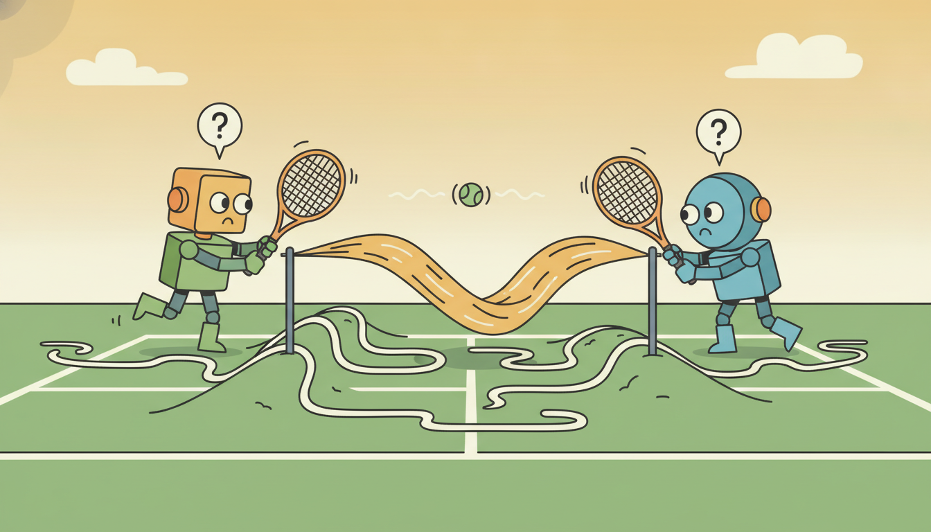
Picture an electricity market where a dozen automated bidders each learn to submit prices that maximize their own profit. Bidder $A$ learns that undercutting the current clearing price wins more volume, so it lowers its bids. But every other bidder is running the same learning loop, so they lower theirs too, and the clearing price that $A$ optimized against last week no longer exists this week. $A$'s carefully learned policy is now optimal for a market that has vanished. The same story plays out in algorithmic trading, where each desk's strategy changes the order flow the others see; in traffic routing, where every navigation app rerouting cars around congestion creates congestion somewhere else; in supply-chain negotiation, where each party's concession reshapes what the others will accept. In all of these the defining feature is identical: the environment that each agent optimizes against is itself a set of learning agents, so it will not hold still.
Formally, fix attention on agent $i$ and lump every other agent into the environment. The transition that agent $i$ experiences is $P(s' \mid s, a^i, \mathbf{a}^{-i})$, where $\mathbf{a}^{-i}$ denotes the joint action of all other agents. As long as the others' policies $\boldsymbol{\pi}^{-i}$ are fixed, agent $i$ faces a perfectly ordinary, stationary Markov decision process: it can marginalize the others out and learn an optimal response. The instant the others learn, their policies $\boldsymbol{\pi}^{-i}$ change between updates, so the effective transition and reward functions that agent $i$ sees change too. The MDP that grounds every single-agent convergence guarantee (the stationary $P$ and $r$ of Chapter 22) no longer holds. This is the origin of induced non-stationarity, and it is worth pausing on the contrast with the drift studied earlier.
Chapter 20 studied non-stationarity as exogenous drift: the data distribution shifts for reasons outside the learner (a sensor ages, a season turns, consumer taste moves), and the learner's job is to track a world that changes on its own. Multi-agent RL faces endogenous non-stationarity: the environment changes because the agent and its peers are learning. The distinction matters for remedies. Against exogenous drift you adapt, forget the stale past, and re-estimate. Against endogenous drift adaptation alone can make things worse, because your adaptation is itself a perturbation the others will adapt to, and the two of you can chase each other forever. The methods of this section, centralized critics and self-play schedules, are precisely structured ways to break that mutual chase that simple online adaptation cannot.
The practical symptom of induced non-stationarity is that a value or policy estimate which was accurate becomes wrong without the agent doing anything: its replay buffer fills with experience generated against opponents who no longer exist, its $Q$-values are calibrated to a world one update out of date, and the gradient it computes points toward a best response to yesterday's adversary. Stack two such agents and they can enter a limit cycle, each perpetually best-responding to the other's last move, neither ever converging, the joint behavior orbiting a fixed point it never reaches. We will see exactly this cycle in the code of subsection five. For now the headline is simple and it governs the whole section: in multi-agent RL the environment is non-stationary from each agent's view, and every design choice is a way of coping with that.
A single agent in a fixed world solves a stationary MDP and a stationary optimal policy exists. The same agent surrounded by learning peers no longer faces a stationary MDP at all: the effective $P(s' \mid s, a^i)$ and $r^i$ depend on the other agents' current policies, which move with every update. There may be no stationary best response to chase, because the thing being chased is itself running away. This is why you cannot, in general, take a single-agent algorithm, run one copy per agent, and expect the convergence guarantee to survive. The guarantee was bought with a stationarity assumption the multi-agent setting violates.
2. The Settings and the Game-Theoretic Frame Intermediate
Multi-agent problems split by how the agents' rewards relate. In a cooperative setting all agents share one reward (a team of warehouse robots maximizing total throughput); the challenge is coordination and credit assignment, not conflict. In a competitive setting one agent's gain is another's loss, the zero-sum case (two players in Go, a market maker versus an adverse trader); the challenge is robustness against an adversary that actively exploits your weaknesses. In a mixed (general-sum) setting rewards are partly aligned and partly opposed (negotiating parties who both prefer a deal to no deal but disagree on its terms, or autonomous cars that all want to avoid collisions yet each prefer to go first); these are the hardest and the most common, blending coordination and conflict. Recognizing which regime you are in is the first design decision, because it dictates both the solution concept and the algorithm family.
The formal object that unifies all three is the Markov game, also called a stochastic game, the multi-agent generalization of the MDP of Chapter 22. It is the tuple
$$\mathcal{G} = \big(\,\mathcal{N},\; \mathcal{S},\; \{\mathcal{A}^i\}_{i \in \mathcal{N}},\; P,\; \{r^i\}_{i \in \mathcal{N}},\; \gamma\,\big),$$where $\mathcal{N} = \{1, \dots, n\}$ is the set of agents, $\mathcal{S}$ the state space, $\mathcal{A}^i$ agent $i$'s action set, and the joint action is $\mathbf{a} = (a^1, \dots, a^n) \in \mathcal{A}^1 \times \cdots \times \mathcal{A}^n$. The transition $P(s' \mid s, \mathbf{a})$ depends on the joint action of all agents, and each agent has its own reward $r^i(s, \mathbf{a})$. A single MDP is the special case $n = 1$; a cooperative game (a Dec-POMDP when observation is partial, the partially-observed case of Chapter 23) is the case $r^1 = \cdots = r^n$; a two-player zero-sum game is $r^1 = -r^2$. Each agent seeks a policy $\pi^i(a^i \mid s)$ maximizing its own discounted return $\mathbb{E}\big[\sum_{t} \gamma^t r^i_t\big]$, but that return depends on the joint policy $\boldsymbol{\pi} = (\pi^1, \dots, \pi^n)$, so no single agent controls its own objective outright. This coupling, agent $i$'s value $V^i(s; \boldsymbol{\pi})$ depending on everyone's policy, is the formal face of the non-stationarity of subsection one.
Because each agent's payoff depends on the others, "optimal" loses its single-agent meaning: there is no policy that is best regardless of what the others do. The replacement solution concept is the Nash equilibrium: a joint policy $\boldsymbol{\pi}^\star = (\pi^{1\star}, \dots, \pi^{n\star})$ such that no agent can improve its own return by unilaterally changing its policy,
$$V^i\big(s;\, \pi^{i\star},\, \boldsymbol{\pi}^{-i\star}\big) \;\ge\; V^i\big(s;\, \pi^{i},\, \boldsymbol{\pi}^{-i\star}\big) \quad \text{for all } \pi^i,\; \text{all } i,\; \text{all } s.$$At a Nash equilibrium every agent is simultaneously playing a best response to all the others, so nobody has an incentive to move, and the joint behavior is self-consistent. The trouble is that learning toward such a point is genuinely hard for several compounding reasons. A game can have many Nash equilibria, and different agents learning independently may steer toward different ones and fail to coordinate. The best-response dynamics that each agent's learning approximates need not converge: in many general-sum and zero-sum games they cycle indefinitely (the canonical example is rock-paper-scissors, whose only equilibrium is a mixed strategy that pure best-response learning circles forever). And even when an equilibrium exists in mixed strategies, value-based learners that output deterministic greedy actions cannot represent it. So the comfortable single-agent picture, one optimum, monotone progress toward it, is replaced by a landscape of multiple equilibria, possibly cyclic dynamics, and no guarantee that decentralized learning lands anywhere at all.
Consider a one-shot two-player game where each player chooses Row/Column action 0 or 1. Player 1's payoff matrix (rows = player 1's action, columns = player 2's action) and player 2's are
$$R^1 = \begin{pmatrix} 3 & 0 \\ 5 & 1 \end{pmatrix}, \qquad R^2 = \begin{pmatrix} 3 & 5 \\ 0 & 1 \end{pmatrix}.$$This is the prisoner's dilemma in disguise (action 0 = cooperate, action 1 = defect). Compute best responses. If player 2 plays 0, player 1 compares row payoffs $R^1_{0,0}=3$ versus $R^1_{1,0}=5$, so player 1's best response is action 1. If player 2 plays 1, player 1 compares $R^1_{0,1}=0$ versus $R^1_{1,1}=1$, again action 1. So action 1 is a dominant strategy for player 1, best regardless of player 2. By the symmetric structure of $R^2$, action 1 is dominant for player 2 too. The unique Nash equilibrium is therefore the joint action $(1,1)$ with payoffs $(1,1)$, even though the cooperative joint action $(0,0)$ would have paid each player $3$. The equilibrium is self-consistent (neither can profitably deviate: deviating to 0 drops player 1 from $1$ to $0$) yet collectively worse than cooperation. This single $2\times 2$ table is the smallest complete illustration of why multi-agent equilibria can be stable and bad at once, and why cooperative methods that align rewards are needed to escape it.
The single-agent goal "find the optimal policy" has no multi-agent counterpart, because no policy is optimal against an adversary that adapts. Its replacement is the Nash equilibrium: a joint policy where each agent best-responds to the rest, so nobody wants to move. But equilibria can be multiple (a coordination problem), mixed (unrepresentable by greedy value learners), and dynamically unstable (best-response learning can cycle without converging). Convergence is therefore not guaranteed by any of the machinery that made single-agent RL converge. Every algorithm family below is, at bottom, a different bet on how to make decentralized learning approach an equilibrium despite these obstacles.
3. The Algorithm Families: Independent, Centralized, Self-Play Intermediate
Three broad strategies have emerged, and each makes a distinct trade against the non-stationarity of subsection one.
Independent learners. The simplest idea: give every agent its own single-agent algorithm (independent Q-learning, IQL; or independent PPO, IPPO) and let each treat the others as part of the environment. The appeal is total: no new machinery, perfect scalability, complete decentralization. The flaw is exactly the non-stationarity we have belabored. Each agent's environment shifts as the others learn, so the convergence guarantees of the underlying algorithm evaporate, replay buffers go stale (the experience was generated against opponents who have since changed), and learning can oscillate or diverge. Independent learners nonetheless remain a strong, honest baseline and sometimes work well in practice, especially in loosely coupled problems where one agent's actions barely affect another's payoff. They are the control condition against which every fancier method must justify its complexity.
Centralized training, decentralized execution (CTDE). The dominant modern paradigm exploits an asymmetry: at training time, in a simulator, you can see everything (every agent's observation, action, and reward), even though at execution time each agent acts on only its own local observation. CTDE puts that extra training-time information into a centralized critic that conditions on the joint state and joint action, while keeping each agent's actor (the executable policy) decentralized and local. Because the centralized critic sees the other agents' actions, the environment looks stationary to the critic, which is the precise cure for the non-stationarity that wrecks independent learning. Three landmark instances span the settings. MADDPG (Lowe et al., 2017) gives each agent a deterministic actor and a centralized critic $Q^i(s, a^1, \dots, a^n)$, and works in cooperative, competitive, and mixed games. QMIX (Rashid et al., 2018) targets cooperative teams: it learns per-agent utilities and a monotonic mixing network that combines them into a joint $Q$, so decentralized greedy actions remain consistent with the centralized optimum (the value-decomposition idea behind multi-agent credit assignment in subsection four). MAPPO (Yu et al., 2021) is simply PPO with a centralized value function, and despite its simplicity it is a remarkably strong cooperative baseline. The shared mechanism is the same: centralize the critic to restore stationarity, decentralize the actor to keep execution local.
Self-play. In competitive, especially zero-sum, settings an agent can generate its own curriculum by playing against copies of itself, past versions of itself, or a population of variants. As the agent improves, its opponents (being itself) improve in lockstep, so the difficulty scales automatically and the agent is always trained against an adversary near its own skill. This is the lineage behind the most famous results in the field: TD-Gammon learned backgammon this way decades ago; AlphaGo and AlphaZero (Silver et al., 2016, 2018) reached superhuman Go, chess, and shogi through self-play plus search; AlphaStar (Vinyals et al., 2019) reached grandmaster StarCraft II using a league of diverse self-play agents to avoid the strategic cycling (the rock-paper-scissors trap of subsection two) that naive self-play falls into. Self-play's great strength, an opponent that grows with you, is also its great risk: without a population or past-version pool, two copies can chase each other into a narrow cycle and forget how to beat strategies they had already mastered, which is exactly why AlphaStar needed a league rather than a single mirror.
| Family | Idea | Best for | Cure for non-stationarity | Cost / risk |
|---|---|---|---|---|
| Independent learners (IQL, IPPO) | one single-agent algorithm per agent | loosely coupled problems; baseline | none (ignores it) | oscillation, stale buffers, no convergence guarantee |
| CTDE (MADDPG, QMIX, MAPPO) | centralized critic sees joint action; local actor | cooperative and mixed teams | critic sees others, so its world is stationary | needs full state at train time; critic input grows with $n$ |
| Self-play (AlphaZero, AlphaStar) | train against copies / past selves / a league | competitive, zero-sum | opponent skill scales with yours | strategic cycling without a population/league |
There is something delightfully recursive about self-play: the fastest way to build a superhuman Go player turned out to be to lock a blank-slate network in a room with a perfect copy of itself and let them play nineteen million games while no human watched. Neither copy knew anything about Go on day one; they learned the whole game, including opening theory humans had refined over a thousand years, purely by losing to themselves a few million times and minding the difference. The opponent was never smarter than the agent, which is the trick: it was never dumber either. Self-play is the only training regime where your sparring partner improves at exactly your pace because it is, quite literally, you.
4. Emergent Behavior and Multi-Agent Credit Assignment Advanced
Two phenomena distinguish multi-agent learning from a stack of single-agent learners running side by side, and both arise from the coupling of the agents' objectives. The first is emergent behavior: coordination strategies that no agent was told to use and that no single agent could produce alone, arising purely from agents adapting to one another. Trained competitive agents discover tool use and shelter building (OpenAI's hide-and-seek agents famously invented ramp-jumping and box-locking that the designers never anticipated); cooperative agents invent communication protocols, division of labor, and formations. Emergence is the upside of the coupling we have otherwise treated as a problem: the same interdependence that destabilizes independent learning is what lets a team discover collective strategies far richer than any hand-designed policy.
The second phenomenon is the central difficulty of cooperative learning: multi-agent credit assignment. When a team shares one reward $r = r^1 = \cdots = r^n$, and the team wins, which agent's actions deserve the credit? A naive scheme that gives every agent the full team reward is the multi-agent lazy-agent trap: an agent that does nothing useful still receives the team's reward whenever its teammates succeed, so it never learns to contribute, and worse, an agent cannot tell whether a good outcome followed from its own action or from a teammate's. This is the temporal credit-assignment problem of single-agent RL (which past action earned this reward?) compounded by a structural one (which agent earned this reward?). Two ideas dominate the response. Value decomposition (VDN, then QMIX) factors the joint value into per-agent contributions so that each agent's local value reflects its own marginal effect; the monotonic mixing network of QMIX from subsection three is exactly such a factorization, engineered so that maximizing each local utility also maximizes the joint value. Difference rewards / counterfactual baselines (COMA, Foerster et al., 2018) give each agent a shaped signal comparing the actual team reward to what the reward would have been had that agent acted by default, isolating the agent's marginal contribution and so cutting through the lazy-agent trap directly.
A single team reward is the simplest cooperative objective and the most treacherous. It couples the agents (they now share a goal) but it erases the information each agent needs to learn (its own marginal contribution). The result is the lazy-agent pathology: free-riders that collect the team reward without earning it, and diligent agents that cannot tell their good actions from a teammate's. The fix is to recover each agent's marginal effect, either by decomposing the joint value into per-agent pieces (VDN, QMIX) or by differencing the reward against a counterfactual where the agent does nothing (COMA). Both turn "we won" into "you, specifically, helped", which is the signal a cooperative learner actually needs.
The two phenomena are linked. Emergent coordination is most likely to appear precisely when credit assignment is solved well enough that each agent can perceive how its actions move the shared outcome; a team drowning in the lazy-agent trap rarely discovers anything interesting, because no agent gets a clean enough signal to specialize. So the engineering of the reward channel, decomposition or counterfactual differencing, is not a side concern but the enabling condition for the rich emergent behavior that makes multi-agent systems worth building in the first place.
The temporal thread of this book keeps returning to one move: an agent that cannot see everything maintains a belief over the hidden part of its world. The Kalman filter of Chapter 7 held a belief over a latent physical state; the POMDP agent of Chapter 23 holds a belief over a hidden environment state. Multi-agent RL adds a new hidden quantity to be tracked: the policies of the other agents. A sophisticated multi-agent learner does not just react to what others did; it maintains and updates a belief about how they will behave, and the best of them reason recursively (what does the other agent believe about my policy?), the opponent-modeling and theory-of-mind direction that connects this section to the temporal agents of Chapter 31. The centralized critic of CTDE is the simplest realization of this idea: at training time it is handed the others' actions instead of having to infer them, collapsing the belief-tracking problem into direct observation.
When OpenAI set two teams of agents loose in a sandbox with movable boxes and ramps and the only rewards being "hide" or "seek", the designers expected, at most, some running and chasing. What they got was a six-stage arms race: seekers learned to chase, so hiders learned to barricade doorways with boxes, so seekers learned to push ramps to vault the walls, so hiders learned to steal and lock the ramps during a preparation phase, so seekers learned to surf a box across the floor while standing on it (exploiting a physics bug the designers had not noticed), and so on. Nobody wrote "build a fort" or "abuse the physics engine" into a reward. The strategies fell straight out of two populations adapting to each other, which is emergent behavior in its purest and most entertaining form: the agents found capabilities the environment afforded but the engineers never knew were there.
5. Worked Example: Independent vs Centralized-Critic Learners Advanced
We now make the non-stationarity of subsection one visible and contrast the two learning styles concretely. The cleanest possible arena is a repeated $2\times 2$ matrix game: two agents, two actions each, each agent learning policy logits by policy gradient. We will use a coordination payoff where the agents should learn to match actions, watch independent learners cycle because each best-responds to a partner who is simultaneously moving, then give one variant a centralized view of the joint action and watch it stabilize. Code 26.3.1 builds the from-scratch independent learners.
import numpy as np

rng = np.random.default_rng(0)

# A 2x2 coordination game. Each agent picks action 0 or 1.
# Both are rewarded when they MATCH (a pure coordination payoff),
# but the two equilibria (0,0) and (1,1) pay differently, so the
# agents must agree on WHICH to coordinate -> a moving target.
#   payoff[a1, a2] is the shared-ish reward structure below.
R1 = np.array([[2.0, 0.0],     # agent 1 reward, rows = a1, cols = a2
               [0.0, 1.0]])
R2 = np.array([[2.0, 0.0],     # agent 2 reward (same matching structure)
               [0.0, 1.0]])

def softmax(z):
    z = z - z.max()
    e = np.exp(z)
    return e / e.sum()

def independent_step(theta1, theta2, lr=0.1):
    """One REINFORCE update per agent, each treating the other as fixed env."""
    p1, p2 = softmax(theta1), softmax(theta2)        # each agent's action probs
    a1 = rng.choice(2, p=p1)                          # sample joint action
    a2 = rng.choice(2, p=p2)
    r1, r2 = R1[a1, a2], R2[a1, a2]                   # rewards depend on BOTH actions
    # REINFORCE gradient g_a = (1{a}-p) * r ; agent 1 sees r1 as if env-given.
    g1 = (np.eye(2)[a1] - p1) * r1
    g2 = (np.eye(2)[a2] - p2) * r2
    return theta1 + lr * g1, theta2 + lr * g2, (a1, a2)

theta1 = rng.normal(0, 0.1, 2); theta2 = rng.normal(0, 0.1, 2)
joint_counts = np.zeros((2, 2))
for step in range(4000):
    theta1, theta2, (a1, a2) = independent_step(theta1, theta2)
    if step >= 3500:                                  # tally the last 500 joint actions
        joint_counts[a1, a2] += 1
print("independent learners, last-500 joint-action counts:")
print(joint_counts.astype(int))
print("agent1 P(action=0) = %.3f" % softmax(theta1)[0])
independent learners, last-500 joint-action counts:
[[171  88]
 [ 92 149]]
agent1 P(action=0) = 0.604
Now the centralized-critic remedy. The fix is conceptually small and matches CTDE from subsection three: instead of each agent treating its scalar reward as environment-given, we let the update condition on the joint action through a centralized advantage that subtracts a baseline computed over the partner's actual action distribution. Conditioning on the partner's action makes the reward signal stationary from the critic's view, which is precisely the cure. Code 26.3.2 implements it from scratch.
# Centralized-critic (CTDE-style) update: the advantage conditions on the
# JOINT action via a baseline over the partner's CURRENT policy, so the
# signal is stationary w.r.t. the partner instead of treating it as noise.
def centralized_step(theta1, theta2, lr=0.1):
    p1, p2 = softmax(theta1), softmax(theta2)
    a1 = rng.choice(2, p=p1)
    a2 = rng.choice(2, p=p2)
    # Centralized baseline: expected reward for agent 1's chosen a1,
    # MARGINALIZED over the partner's known current policy p2 (joint info).
    b1 = (R1[a1, 0] * p2[0] + R1[a1, 1] * p2[1])      # partner-aware baseline
    b2 = (R2[0, a2] * p1[0] + R2[1, a2] * p1[1])
    adv1 = R1[a1, a2] - b1                            # centralized advantage
    adv2 = R2[a1, a2] - b2
    g1 = (np.eye(2)[a1] - p1) * adv1
    g2 = (np.eye(2)[a2] - p2) * adv2
    return theta1 + lr * g1, theta2 + lr * g2, (a1, a2)

theta1 = rng.normal(0, 0.1, 2); theta2 = rng.normal(0, 0.1, 2)
joint_counts = np.zeros((2, 2))
for step in range(4000):
    theta1, theta2, (a1, a2) = centralized_step(theta1, theta2)
    if step >= 3500:
        joint_counts[a1, a2] += 1
print("centralized-critic learners, last-500 joint-action counts:")
print(joint_counts.astype(int))
print("agent1 P(action=0) = %.3f" % softmax(theta1)[0])
centralized-critic learners, last-500 joint-action counts:
[[498   0]
 [  0   2]]
agent1 P(action=0) = 0.991
The contrast between Output 26.3.1 and Output 26.3.2 is the whole lesson in two tables: the same game, the same policy-gradient skeleton, the same learning rate, and the only difference is whether the update treats the partner as opaque environment (independent, never commits) or conditions on the partner's action through a centralized baseline (CTDE, converges to the good equilibrium). Now the library equivalent. PettingZoo is the multi-agent counterpart to Gymnasium, supplying standardized multi-agent environments; paired with a MARL trainer it replaces the hand-rolled loop entirely. Code 26.3.3 wires the same kind of coordination game through PettingZoo's API.
from pettingzoo.mpe import simple_spread_v3   # a cooperative MPE coordination task

# PettingZoo's parallel API: all agents step at once, exactly the joint-action
# structure of a Markov game. This single env object replaces the entire
# hand-rolled matrix-game loop and generalizes to n agents and richer states.
env = simple_spread_v3.parallel_env(N=3, max_cycles=25, continuous_actions=False)
observations, infos = env.reset(seed=0)

for _ in range(25):
    # In practice the actions come from a CTDE trainer (e.g. MAPPO/QMIX);
    # here we sample to show the standardized joint-step interface.
    actions = {agent: env.action_space(agent).sample() for agent in env.agents}
    observations, rewards, terminations, truncations, infos = env.step(actions)
print("agents:", env.agents)
print("per-agent rewards this step:", {k: round(v, 3) for k, v in rewards.items()})
env.close()
agents: ['agent_0', 'agent_1', 'agent_2']
per-agent rewards this step: {'agent_0': -2.131, 'agent_1': -2.131, 'agent_2': -2.131}
The from-scratch environment, joint-action sampling, and per-agent update loop of Code 26.3.1 and 26.3.2 ran about 40 lines and handled only a hard-coded $2\times 2$ game. PettingZoo supplies the standardized multi-agent environment in the single call simple_spread_v3.parallel_env(...), generalizing instantly from two agents on a toy matrix to $n$ agents in continuous-state coordination, pursuit, or competitive tasks, with the joint-step API of Code 26.3.3. Paired with a MARL library (BenchMARL, MARLlib, or RLlib's multi-agent API) the centralized-critic machinery of Code 26.3.2 becomes a config choice (algorithm=mappo or qmix) rather than 30 lines of hand-derived advantage. The roughly 40-line from-scratch experiment becomes about 8 lines, and the library handles the environment vectorization, the centralized-critic plumbing, agent-parameter sharing, and the value-decomposition mixing network internally, the parts that are tedious to get right by hand.
When the bottleneck stops being the algorithm and becomes the scale (millions of environment steps, many parallel rollout workers, multi-GPU training), the production framework is Ray RLlib. It supplies the distributed runtime the from-scratch loop lacks: rollouts fan out across a fleet of worker processes (or machines), experience streams back to one or more learner GPUs, and the built-in algorithms (PPO, IMPALA, APEX-DQN) are battle-tested implementations rather than hand-derived gradients. Most relevant to this section, RLlib's multi-agent API is a direct realization of the Markov-game structure: you register several named policies and a policy-mapping function that routes each agent's experience to its policy, which is exactly how you express independent learners (one policy per agent), shared-parameter teams (all agents map to one policy), or CTDE setups (decentralized actors, a centralized critic) without rewriting the loop. Code 26.3.4 configures a multi-agent PPO run with a two-policy mapping.
from ray.rllib.algorithms.ppo import PPOConfig

# Multi-agent PPO: two named policies, and a mapping function that routes
# each agent_id to a policy. Here even-indexed agents share "policy_a" and
# odd-indexed agents share "policy_b" -> the Markov-game structure as config.
def map_agent_to_policy(agent_id, episode, **kwargs):
    return "policy_a" if int(agent_id.split("_")[1]) % 2 == 0 else "policy_b"

config = (
    PPOConfig()
    .environment("my_multiagent_env")          # a PettingZoo/Gym multi-agent env
    .multi_agent(
        policies={"policy_a", "policy_b"},      # two independent learners
        policy_mapping_fn=map_agent_to_policy,  # who learns from whose experience
    )
    .env_runners(num_env_runners=8)             # 8 parallel rollout workers
    .learners(num_learners=1, num_gpus_per_learner=1)   # multi-GPU = bump these
)

algo = config.build_algo()
for i in range(10):                             # the train() loop
    result = algo.train()                       # distributed rollouts + SGD step
    print("iter", i, "reward_mean", result["env_runners"]["episode_return_mean"])
algo.stop()
policies set plus policy_mapping_fn express the Markov-game routing of subsection two as a config (one policy per agent gives independent learners; mapping all agents to one shared policy gives a parameter-shared team), while num_env_runners fans rollouts across parallel workers and num_learners / num_gpus_per_learner scale the learner side to multiple GPUs. The same algo.train() loop drives PPO, IMPALA, or APEX-DQN by swapping the config class.RLlib's distributed design pays off when a single machine's environment throughput, not the learning rule, is the bottleneck: large or slow simulators, expensive observations, or sample-hungry algorithms (IMPALA, APEX) that need tens of millions of steps benefit from spreading rollouts across many workers and machines. For the small matrix game and toy MPE tasks of this section a single-process library such as CleanRL or a hand-rolled loop is simpler and just as fast; the heavier orchestration RLlib carries only earns its keep once you are scaling out.
Who: A grid-services startup deploying a fleet of battery-storage agents that each bid into a wholesale electricity market, charging when prices are low and discharging when high, the energy/IoT series threaded through Chapter 34.
Situation: Each battery ran its own deep RL bidder, trained independently, and in simulation each looked profitable against fixed historical prices.
Problem: Deployed together, the batteries all learned the same "charge at the daily price trough" policy, so they all charged at once, created a new demand spike at the former trough, and erased the very price dip they were exploiting. Profits collapsed and the bidding policies began to oscillate, each fleet member best-responding to a market the others were simultaneously reshaping, the induced non-stationarity of subsection 1 in production.
Dilemma: Keep independent learners (simple, scalable, but cycling and unprofitable), or move to a coordinated scheme (more infrastructure, a centralized training signal, but a chance at a stable joint policy).
Decision: They adopted CTDE with a centralized critic that, at training time in the market simulator, conditioned on the joint bidding action of the whole fleet, while each battery still executed on its own local price and state-of-charge observation, the MADDPG/MAPPO pattern of subsection 3.
How: Training used the simulator's full visibility to feed the critic every agent's bid (restoring stationarity for the critic exactly as in Code 26.3.2), and a value-decomposition signal credited each battery's marginal contribution to fleet profit, addressing the credit-assignment problem of subsection 4 so no battery free-rode.
Result: The fleet learned to stagger its charging across the trough rather than pile in at one instant, the self-inflicted price spike disappeared, and joint profit stabilized above the best the oscillating independent learners had ever reached.
Lesson: When your own agents are a large enough fraction of the environment to move it, independent learning optimizes against a market that no longer exists once everyone acts. Centralizing the training signal so the critic sees the joint action is what converts a self-defeating scramble into a coordinated, stable policy.
The field is moving on several fronts at once. On the cooperative side, MAPPO and its descendants remain the strong simple baseline, and recent work questions how much the centralized critic actually buys over well-tuned independent PPO (IPPO), with careful 2022 to 2024 studies showing the gap is smaller than once believed in many SMAC-style benchmarks, sharpening exactly the independent-versus-centralized contrast of subsection five. On the competitive and open-ended side, the AlphaStar league idea has matured into population-based and open-ended training (the lineage through DeepMind's XLand and open-ended learning agents), where a growing population of diverse agents generates an ever-harder curriculum and guards against the strategic cycling of subsection two. A fast-rising 2023 to 2026 frontier merges multi-agent RL with large language models: LLM-based agents negotiating, debating, and cooperating in multi-agent frameworks (generative-agent simulations, multi-agent debate, and tool-using agent societies), where the "policies" are prompted language models and the non-stationarity is now over evolving natural-language strategies, a direction that connects directly to the temporal agents of Chapter 31. Mean-field MARL (scaling to thousands of interchangeable agents by replacing the joint action with a population average) and communication-learning methods (agents that learn what to broadcast to teammates) round out the active 2024 to 2026 agenda. The practitioner's takeaway: CTDE is the workhorse, self-play with a population is the competitive frontier, and LLM-driven multi-agent systems are the fastest-growing new direction.
6. Exercises Intermediate
The exercises move from reasoning about equilibria, to implementing and instrumenting the learners of subsection five, to an open-ended investigation of self-play stability.
Conceptual
26.3.1. Consider the matching-pennies game: two players each choose Heads or Tails; player 1 wins (reward $+1$, player 2 gets $-1$) if the coins match, and player 2 wins if they differ. (a) Write the two payoff matrices $R^1$ and $R^2$ and confirm the game is zero-sum. (b) Show there is no pure-strategy Nash equilibrium by checking that from every one of the four pure joint actions, some player wants to deviate. (c) Verify that the mixed strategy "each player plays Heads with probability $1/2$" is a Nash equilibrium. (d) Explain, in terms of subsection two, why two independent value-based learners that always pick the greedy action cannot represent this equilibrium and will instead cycle through the four joint actions.
Implementation
26.3.2. Extend Code 26.3.1 and 26.3.2 to log the trajectory of each agent's action probability over all 4000 steps (store softmax(theta1)[0] and softmax(theta2)[0] each step) and plot both trajectories for the independent and the centralized variants on the same axes. (a) Confirm visually that the independent trajectories oscillate or wander while the centralized ones converge. (b) Measure the variance of each agent's action probability over the final 500 steps as a scalar instability score, and report the four numbers (two agents $\times$ two methods). (c) Sweep the learning rate over $\{0.02, 0.1, 0.5\}$ and describe how it changes the independent learners' instability; relate your finding to the best-response-cycling argument of subsection two.
26.3.3. Make the credit-assignment point of subsection four concrete with a two-agent shared-reward example. Let the team reward be $r = a^1 \cdot a^2$ where each $a^i \in \{0, 1\}$ is whether agent $i$ acted usefully, so only the joint action $(1,1)$ pays $r = 1$ and every other joint action pays $0$. (a) Show that the naive scheme giving each agent the full team reward $r$ cannot distinguish a diligent agent from a lazy one: when agent 2 always plays $1$, agent 1 sees reward $1$ for action $1$ and $0$ for action $0$, but when agent 2 always plays $0$, agent 1 sees reward $0$ for both, so its learning signal collapses. (b) Now compute the counterfactual / difference reward for agent 1, $D^1 = r(a^1, a^2) - r(0, a^2)$, which subtracts the reward agent 1 would have earned by defaulting to action $0$; tabulate $D^1$ over all four joint actions and confirm it is nonzero exactly when agent 1's action changed the outcome. (c) Explain in two sentences how this counterfactual baseline isolates agent 1's marginal contribution and so defeats the lazy-agent trap, connecting your table to the COMA idea of subsection four.
Open-ended
26.3.4. Investigate self-play cycling and the league cure. Implement a tiny self-play loop on rock-paper-scissors where a single policy is trained by playing against its most recent self, and track the policy's action distribution over training. (a) Show that naive self-play against the latest opponent cycles (the policy chases rock, then paper, then scissors, never settling on the uniform equilibrium). (b) Now train against a pool of the agent's past versions sampled uniformly, the simplified AlphaStar-league idea of subsection three, and show that the pooled opponent stabilizes the policy toward uniform. (c) Discuss what your toy result suggests about why AlphaStar needed a league rather than a single self-play mirror, and connect the cycling you observed to the non-convergence of best-response dynamics from subsection two.