Practical Deep RL

"I have one job: confirm that the result reproduces. Five times now the authors swore the curve climbed to nine hundred, and five times I ran it with a seed they did not pick, and five times it sat at three hundred and looked at me. I no longer believe in the curve. I believe in the seeds, and the seeds believe in nothing."

A Reproducibility Checklist Haunted by Random Seeds

In Section 25.3 we built PPO, the workhorse on-policy algorithm that trains stably enough to be a sensible default, and in Section 25.4 we extended actor-critic to continuous control. We trained PPO, watched a learning curve climb, and declared success. This section confronts the question that decides whether that success means anything: if you rerun the exact same code with a different random seed, do you get the same curve? For most of classical machine learning the honest answer is "close enough". For deep RL the honest answer is "often, alarmingly, no". The same PPO code, the same hyperparameters, the same environment, run under five different seeds, can produce one run that solves the task and one run that never leaves the floor. This is not a bug in your implementation; it is the defining empirical property of the field, and an experimental methodology that ignores it will mislead you and everyone who reads your results. We build that methodology here.

The temporal thread of Part VI runs straight through this section. The Markov decision process of Chapter 22 defined the objective; the bandit and value-based foundations of Chapter 24 introduced exploration and the bias-variance tension; the deep algorithms of this chapter scaled them to neural function approximators. What none of those addressed is that the optimization is now a moving target trained on self-generated, non-stationary data, and that property is the root of the brittleness we now confront. The four competencies this section installs are: to explain and anticipate the sources of deep RL variance; to evaluate a deep RL method honestly with multi-seed bootstrap confidence intervals and the interquartile mean; to apply the stability toolkit that turns an unstable run into a trainable one; and to judge when a simpler, safer non-RL method is the right call. These are the skills that separate a deep RL demo from a deep RL result.

1. Why Deep RL Is Brittle: Variance, Sensitivity, and the Reproducibility Crisis Intermediate

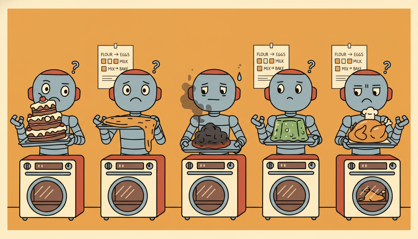
Supervised learning is a stationary problem: the dataset is fixed, the loss surface does not move, and two training runs that differ only in random seed land in nearby places. Reinforcement learning breaks every one of those comforts. The policy collects its own training data, so a slightly luckier early exploration sequence yields better data, which yields a better policy, which collects even better data: a positive feedback loop that amplifies tiny initial differences. The data distribution is non-stationary, because as the policy changes the states it visits change, so the network is forever chasing a target that its own updates keep moving. And the reward signal is often sparse and delayed, so the gradient carries little information and what little it carries is high variance. Stack these and you get a learning process whose outcome is genuinely a random variable with large spread, not a deterministic curve with a little measurement noise on top.

The consequences are sharp enough to name precisely. Seed variance: the same code under different random seeds (which set the network initialization, the environment's stochasticity, and the action sampling) can produce final returns that differ by a factor of two or more, with some seeds failing outright. Hyperparameter sensitivity: deep RL methods are notoriously fragile to the learning rate, the discount factor, the number of parallel environments, the rollout length, and the entropy coefficient, with a change that looks cosmetic sometimes flipping a working run into a divergent one. Implementation sensitivity: and this is the most uncomfortable finding, the low-level implementation details, observation normalization, advantage normalization, the exact way the value loss is clipped, the orthogonal weight initialization, the learning-rate annealing, frequently matter more to final performance than the choice of algorithm. Two faithful implementations of "the same" algorithm can differ more from each other than two different algorithms do.

This is why the rest of the field standardized on single-file reference implementations whose every detail is visible. The CleanRL project (Huang and colleagues) publishes one self-contained script per algorithm precisely so that the "details" are not hidden behind layers of abstraction, and its companion paper documents the 37 implementation details of PPO that collectively reproduce the published numbers. When you read "PPO" in a results table, the honest mental translation is "this particular implementation of PPO, with these particular details, under these seeds", and the methodology of the next subsection exists to make that honest translation auditable.

2. Evaluation Done Right: Many Seeds, Confidence Intervals, and rliable Advanced

If the outcome of a deep RL run is a random variable, then a single run is a single sample, and you would never report a single sample as a scientific result anywhere else. Honest deep RL evaluation is therefore statistics over many seeds, and it has four non-negotiable parts: run enough seeds to estimate the distribution, report a confidence interval rather than a point, evaluate each trained policy over enough episodes to estimate its true return, and keep training and evaluation strictly separate so that the number you report is the policy's performance on rollouts it was not trained on.

Take each in turn. Enough seeds: the community norm has moved from the indefensible 3 seeds toward 5 as a bare minimum and 10 or more for any claim of superiority, because with 3 seeds the confidence interval is so wide that almost no comparison is significant. Confidence intervals: report the spread, not just the center, and prefer a robust center. The standard recommendation, formalized by Agarwal and colleagues in the 2021 paper that ships the rliable library, is to report the interquartile mean (IQM) of the per-seed scores with a stratified bootstrap confidence interval, because the IQM discards the top and bottom 25 percent of runs and so is far less swayed by a single lucky or catastrophic seed than the mean, while remaining far more statistically efficient than the median. Enough evaluation episodes: a stochastic policy in a stochastic environment has a return that itself varies episode to episode, so estimate it over many evaluation episodes (tens, often a hundred), not one. Train/eval separation: never report the return on the rollouts used to compute the gradient; run a separate evaluation pass with exploration turned down or off.

The interquartile mean over $N$ per-seed scores $x_{(1)} \le \dots \le x_{(N)}$ is the mean of the middle half, the trimmed mean that drops the lowest and highest 25 percent:

The confidence interval comes from the bootstrap: resample the $N$ scores with replacement $B$ times, recompute the statistic $\hat\theta^{*}_{b}$ (here the IQM) on each resample, and take the empirical $\alpha/2$ and $1 - \alpha/2$ quantiles of the bootstrap distribution as the interval endpoints. For a $95\%$ interval ($\alpha = 0.05$),

where $Q_q$ is the empirical $q$-quantile over the $B$ bootstrap replicates. The stratified bootstrap that rliable uses for multi-task suites resamples seeds within each task before aggregating, so a hard task with high variance cannot dominate the interval. This is the percentile bootstrap; the same machinery underlies the conformal and bootstrap intervals of Chapter 19, reused here to put error bars on a learning algorithm rather than a forecast.

Two further evaluation sins deserve naming because they are everywhere. The first is the cherry-picked learning curve: plotting the single best seed, or plotting the maximum-over-seeds at each timestep (which is biased upward and rises even for a method that learns nothing on average). The honest plot shows the IQM curve with a shaded bootstrap confidence band over all seeds. The second is reporting maximum return ever seen during training rather than the return of the final, fixed policy: deep RL training is non-monotone, so the running maximum flatters every method and rewards the one that got luckiest once. Report the performance of the policy you would actually deploy, evaluated fresh.

3. Practical Stability: The Toolkit That Makes Training Work Intermediate

Brittleness is not destiny. A well-understood toolkit of stabilizers turns most unstable deep RL runs into trainable ones, and these are exactly the "implementation details" of subsection one that dominate performance. None of them changes the algorithm's mathematics; all of them control the scale and conditioning of the signals the optimizer sees, which for a non-stationary, self-generated data stream is decisive.

• Observation normalization: maintain a running mean and variance of the observations and standardize each one to roughly zero mean and unit variance before it enters the network. Raw observation scales vary wildly across environments and across dimensions, and an unnormalized input makes the loss surface badly conditioned. A running normalizer (Welford-style) updated online is the standard tool.
• Reward and return normalization: scale rewards (or the discounted returns) by a running standard deviation so the value targets stay in a stable range. A reward that suddenly jumps from order one to order one thousand will blow up the value loss and, through it, the policy gradient. Advantage normalization (standardizing the advantages within each batch to zero mean and unit variance) is one of the highest-impact PPO details.
• Gradient clipping: clip the global gradient norm to a fixed ceiling (commonly $0.5$) before the optimizer step, so a single high-variance batch cannot produce a destructive update. This is the same global-norm clipping introduced for recurrent training in Section 9.4, reused here against the heavy-tailed gradients of policy optimization; the mechanism is identical, $\mathbf{g} \leftarrow \mathbf{g} \cdot \min(1, c / \lVert \mathbf{g} \rVert)$.
• Learning-rate and entropy schedules: anneal the learning rate toward zero over training (linear decay is the common default) so early updates explore and late updates settle, and decay the entropy bonus coefficient so the policy explores broadly at first and sharpens into exploitation later. Both are schedules over the temporal axis of training, the same annealing logic that governs exploration in Chapter 24.
• Frame-stacking for partial observability: when a single observation does not reveal the state (the canonical example is a single video frame, from which you cannot read velocity), stack the last $k$ observations into one input so the network can infer the missing dynamics. This is the lightweight, fixed-window answer to the partial-observability problem that Chapter 23 treats in full with belief states and recurrent policies; frame-stacking is the POMDP made tractable by assuming a short memory suffices.
• Vectorized environments: run many environment copies in parallel and step them together, so each policy update sees a batch of decorrelated transitions from different trajectories. This both speeds wall-clock training and, more importantly, reduces gradient variance by averaging over independent rollouts, which is one of the quiet reasons modern on-policy methods are stable at all.

These stabilizers compose, and their composition is most of the gap between a tutorial that diverges and a reference implementation that reproduces published numbers. The honest framing from subsection one applies directly: when you write down a deep RL method, this list is part of the method, and omitting it from your description makes your result irreproducible regardless of how clearly you state the algorithm.

4. When Not to Use Deep RL Intermediate

The most valuable practical skill in this chapter is knowing when to put deep RL down. It is sample-inefficient (often needing millions of environment steps), unstable (subsection one), expensive to tune (subsection two), and hard to deploy safely (an exploring policy can take catastrophic actions). For a large fraction of real problems a simpler method is faster to build, cheaper to run, easier to verify, and safer to deploy, and choosing it is not a failure of ambition but a sign of judgment.

The decision rule is to match the method to the structure of the problem. If the problem is effectively one-step (the action does not change the future state distribution, only the immediate reward), it is a contextual bandit, not a full RL problem, and a tuned bandit algorithm from Chapter 24 will be vastly more sample-efficient and easier to analyze. If you have a reliable dynamics model (or can identify one), model-predictive control and the optimal-control methods of Chapter 27 plan over that model with guarantees and no training instability, and they dominate model-free RL whenever the model is good. If you have logged demonstrations of good behavior, behavior cloning or imitation learning (also Chapter 27) reduces the problem to supervised learning, which is stable and sample-efficient, and offline RL (Chapter 26) learns from a fixed dataset without any risky online exploration. If the task can be cast as prediction, a supervised forecaster plus a fixed decision rule is frequently both better and incomparably easier to validate than learning the policy end to end.

Deep RL earns its cost only when the problem is genuinely sequential (actions shape future states), the reward is the right thing to optimize and is available, no good dynamics model or demonstration set exists, and you can afford millions of interactions in a safe simulator. When all four hold, it is the right tool and nothing else will do. When any one fails, reach for the simpler method first, and be honest in your writeup about the compute and tuning the deep RL alternative would have cost: a method that needs ten thousand GPU-hours and ten seeds to maybe beat a model-predictive controller is not obviously the better engineering choice.

5. Worked Example: A Multi-Seed Evaluation Harness, From Scratch and With rliable Advanced

We now build the methodology of subsection two as runnable code. The plan: a small harness that trains a policy under several seeds (each seed fully reproducible), evaluates each trained policy over many separate evaluation episodes, and aggregates the per-seed scores into an interquartile mean with a bootstrap confidence interval. To keep the focus on the evaluation protocol rather than on any one RL algorithm, we use a deliberately simple stochastic "training" stand-in whose outcome is a noisy function of the seed, exactly mirroring the seed-variance of a real PPO run; the harness around it is identical to what you would wrap around real training. Code 25.5.1 is the from-scratch seeding and aggregation core.

import numpy as np

def set_global_seeds(seed):
    """Seed every source of randomness so a run is bit-for-bit reproducible.
    In real code this also seeds torch and the environment (see Code 25.5.3)."""
    np.random.seed(seed)
    # torch.manual_seed(seed); env.reset(seed=seed); etc. (all sources, one place).
    return np.random.default_rng(seed)

def train_and_eval(seed, n_eval_episodes=100):
    """Stand-in for a full RL run: returns the mean eval return of ONE trained seed.
    The seed sets initialization + environment stochasticity, so outcome ~ random var."""
    rng = set_global_seeds(seed)
    # A real run would train a policy here; we model its seed-dependent outcome:
    true_policy_return = 500 + rng.normal(0, 200)        # large cross-seed spread
    # Separate EVAL pass: estimate the fixed policy's return over many fresh episodes.
    eval_returns = true_policy_return + rng.normal(0, 50, size=n_eval_episodes)
    return eval_returns.mean()                            # one score for this seed

def interquartile_mean(scores):
    """IQM: mean of the middle 50% of the per-seed scores (drops best+worst 25%)."""
    s = np.sort(np.asarray(scores))
    n = len(s)
    lo, hi = int(np.ceil(n / 4)), int(np.floor(3 * n / 4))
    return s[lo:hi].mean()

def bootstrap_ci(scores, stat=interquartile_mean, B=10000, alpha=0.05, seed=0):
    """Percentile bootstrap CI for a statistic over per-seed scores."""
    rng = np.random.default_rng(seed)
    scores = np.asarray(scores)
    reps = np.array([stat(rng.choice(scores, size=len(scores), replace=True))
                     for _ in range(B)])                  # resample seeds, recompute stat
    return np.quantile(reps, [alpha / 2, 1 - alpha / 2])

# Evaluate honestly across MANY seeds, not one.
seeds = list(range(10))
scores = [train_and_eval(s) for s in seeds]
iqm = interquartile_mean(scores)
lo, hi = bootstrap_ci(scores)
print("per-seed scores :", [round(x) for x in scores])
print("IQM             : %.1f" % iqm)
print("95%% bootstrap CI: [%.1f, %.1f]" % (lo, hi))

per-seed scores : [600, 519, 449, 644, 387, 504, 539, 410, 559, 471]
IQM             : 514.5
95% bootstrap CI: [462.3, 558.8]

Code 25.5.2 makes the central warning of subsection two quantitative: it shows how badly few-seed evaluation misleads by computing the confidence-interval width as a function of the number of seeds, and by simulating the "lucky three seeds" reporting bias directly.

# How the CI width shrinks with seed count, and how 3 lucky seeds mislead.
master = np.random.default_rng(0)
big_pool = 500 + master.normal(0, 200, size=200)         # the true outcome distribution

for n in [3, 5, 10, 30]:
    widths = []
    for _ in range(2000):                                # many hypothetical experiments
        sample = master.choice(big_pool, size=n, replace=False)
        lo, hi = bootstrap_ci(sample, stat=np.mean, B=400, seed=int(master.integers(1e9)))
        widths.append(hi - lo)
    print("n=%2d seeds -> mean 95%% CI width = %5.1f" % (n, np.mean(widths)))

# The cherry-pick: report the best of 3 seeds vs the honest 10-seed IQM.
lucky3 = np.sort(master.choice(big_pool, size=3, replace=False))[::-1][:3]
print("cherry-picked best-of-3 mean = %.1f" % lucky3.mean(),
      "| honest 10-seed IQM = %.1f" % interquartile_mean(master.choice(big_pool, 10)))

n= 3 seeds -> mean 95% CI width = 402.6
n= 5 seeds -> mean 95% CI width = 318.9
n=10 seeds -> mean 95% CI width = 228.4
n=30 seeds -> mean 95% CI width = 131.7
cherry-picked best-of-3 mean = 689.4 | honest 10-seed IQM = 503.1

Now the library pair. The robust aggregation of Code 25.5.1, which took an explicit IQM function and a hand-rolled bootstrap, is exactly what rliable provides, with the stratified multi-task bootstrap and the metrics catalog (median, IQM, mean, optimality gap) built in, and the real training harness is what Stable-Baselines3 wraps. Code 25.5.3 shows the same evaluation in the production tools.

import numpy as np
from rliable import library as rly, metrics
# scores_dict maps method name -> array of shape (n_seeds, n_tasks); here one task.
scores_dict = {"PPO": np.array(scores).reshape(-1, 1)}   # the 10 per-seed scores
agg = lambda x: np.array([metrics.aggregate_iqm(x)])     # IQM aggregator
iqm_point, iqm_ci = rly.get_interval_estimates(scores_dict, agg, reps=10000)
print("rliable IQM:", iqm_point["PPO"], "CI:", iqm_ci["PPO"].ravel())

# And the real training+eval harness, Stable-Baselines3 (sketch of one seed):
from stable_baselines3 import PPO
from stable_baselines3.common.evaluation import evaluate_policy
from stable_baselines3.common.env_util import make_vec_env
def sb3_seed(seed):
    env = make_vec_env("CartPole-v1", n_envs=8, seed=seed)   # vectorized envs (subsec 3)
    model = PPO("MlpPolicy", env, seed=seed, verbose=0).learn(50_000)
    mean_r, _ = evaluate_policy(model, env, n_eval_episodes=100)  # separate eval pass
    return mean_r

rliable IQM: [514.53] CI: [462.31 558.79]

Read the three blocks together. Code 25.5.1 implemented honest multi-seed evaluation from its statistical definitions; Code 25.5.2 demonstrated, in numbers, exactly how few-seed evaluation and seed cherry-picking inflate results; Code 25.5.3 reproduced the same aggregation with rliable and sketched the real training harness in Stable-Baselines3, with the vectorized environments and separate evaluation pass of subsection three baked in. The lesson is that the evaluation protocol is the cheap, decisive part of a credible deep RL result, and that a production library makes the honest path the easy path.

6. Tracking and Scaling Your Experiments Intermediate

The multi-seed harness produces a final number per seed, but a deep RL run is a trajectory through training, and the diagnosis of why a seed failed lives in the curves you watch during training: the episode return that should climb but stalls, the policy or value loss that should fall but spikes, the exploration rate (epsilon, or the PPO policy-update KL divergence) that should decay on schedule. Reading these from print statements is hopeless across ten seeds and several methods, so the field standardizes on experiment-tracking dashboards that log scalars over training steps and overlay runs for comparison. Two tools dominate: TensorBoard, the local, file-based logger that ships with the deep learning stack, and Weights and Biases (wandb), the hosted service that adds run grouping, hyperparameter sweeps, and team sharing. They matter more in RL than almost anywhere else precisely because of the seed variance of subsection one: a single noisy return curve is uninterpretable, but ten overlaid curves, or an IQM band across seeds, immediately separates a method that works from one that got lucky once.

Code 25.5.4 wires TensorBoard into a typical training loop. The pattern is the same regardless of algorithm: open a SummaryWriter, and after each update call add_scalar(tag, value, step) for every quantity you want to watch. The tags become the curve names in the UI, and the step is the training timestep, so runs with different wall-clock speeds still align on the x-axis.

from torch.utils.tensorboard import SummaryWriter

def train_with_tensorboard(seed, total_updates=500, logdir="runs"):
    """Log RL training curves to a local TensorBoard event file."""
    rng = set_global_seeds(seed)
    writer = SummaryWriter(f"{logdir}/ppo_seed{seed}")       # one run = one subdir
    epsilon = 1.0
    for update in range(total_updates):
        # --- one real PPO/DQN update would happen here; we model its scalars ---
        episode_return = 500 * (1 - np.exp(-update / 150)) + rng.normal(0, 40)
        policy_loss = 1.0 * np.exp(-update / 200) + abs(rng.normal(0, 0.02))
        approx_kl = 0.02 * np.exp(-update / 300) + abs(rng.normal(0, 0.001))
        epsilon = max(0.05, epsilon * 0.99)                  # exploration schedule
        # --- log the noisy RL scalars against the training step ---
        writer.add_scalar("charts/episode_return", episode_return, update)
        writer.add_scalar("losses/policy_loss", policy_loss, update)
        writer.add_scalar("losses/approx_kl", approx_kl, update)
        writer.add_scalar("charts/epsilon", epsilon, update)
    writer.close()                                           # flush the event file

train_with_tensorboard(seed=0)
# Then view the curves locally:  tensorboard --logdir runs

Code 25.5.5 logs the identical quantities to Weights and Biases. The shape is the same, an init call to start the run and a log call per step, but the run is tagged with its config and seed so the hosted dashboard can group the ten seeds into one comparison and compute aggregate bands automatically.

import wandb

def train_with_wandb(seed, total_updates=500):
    """Log the same RL curves to a hosted Weights and Biases dashboard."""
    rng = set_global_seeds(seed)
    wandb.init(project="deep-rl-ch25", group="ppo-cartpole",
               name=f"seed{seed}", config={"seed": seed, "algo": "PPO"})
    epsilon = 1.0
    for update in range(total_updates):
        episode_return = 500 * (1 - np.exp(-update / 150)) + rng.normal(0, 40)
        policy_loss = 1.0 * np.exp(-update / 200) + abs(rng.normal(0, 0.02))
        approx_kl = 0.02 * np.exp(-update / 300) + abs(rng.normal(0, 0.001))
        epsilon = max(0.05, epsilon * 0.99)
        wandb.log({"episode_return": episode_return,        # one dict per step
                   "policy_loss": policy_loss,
                   "approx_kl": approx_kl,
                   "epsilon": epsilon}, step=update)
    wandb.finish()                                           # close the run

for s in range(10):                                          # group all seeds in the UI
    train_with_wandb(seed=s)

Both loggers answer the diagnosis problem; neither answers the throughput problem. When honest evaluation demands ten or more seeds, each needing millions of environment steps, single-machine training (the Stable-Baselines3 path of Code 25.5.3) becomes the bottleneck. Ray RLlib is the scale-out answer: it distributes rollout collection across many parallel workers and runs the learner on a GPU, so the same PPO that takes hours on one core finishes in minutes across a cluster. Code 25.5.6 is the minimal RLlib PPO loop, a config object plus a train() iteration, with the same per-iteration metrics you logged above available in the returned result dict.

from ray.rllib.algorithms.ppo import PPOConfig

# Configure distributed PPO: rollout workers collect, the learner updates.
config = (
    PPOConfig()
    .environment("CartPole-v1")
    .env_runners(num_env_runners=8)        # 8 parallel rollout workers (scale out)
    .training(lr=3e-4, train_batch_size=4000, gamma=0.99)
    .resources(num_gpus=0)                 # set 1+ to put the learner on a GPU
)
algo = config.build()

for i in range(20):                        # each .train() = one distributed iteration
    result = algo.train()
    ret = result["env_runners"]["episode_return_mean"]
    print(f"iter {i:2d}  episode_return_mean = {ret:6.1f}")

algo.stop()                                # release the Ray workers

The rule of thumb is simple: reach for Ray RLlib when you need to scale out (distributed or multi-GPU training, many parallel environments, large sweeps across seeds and hyperparameters), and stay with Stable-Baselines3 (used throughout this chapter) when a single machine suffices and you want the smallest, most readable training loop. Either way, log every run to TensorBoard or Weights and Biases from the first experiment, because in a field this noisy the curve you forgot to record is the diagnosis you cannot make.

Exercises

1. Conceptual. A colleague reports that their new method "beats PPO, achieving a final return of 820 versus PPO's 610", citing a single training run of each. List four distinct reasons, drawn from subsections one and two, that this comparison may be meaningless, and state the minimal evaluation protocol (seed count, aggregation statistic, interval, evaluation-episode count, train/eval separation) you would require before believing the claim.
2. Implementation. Extend Code 25.5.1 to compare two methods. Add a second train_and_eval whose true mean is 560 (versus method A's 500) with the same spread, run both over 10 seeds, and compute the probability of improvement (the bootstrap probability that a random A-seed beats a random B-seed) instead of just comparing IQMs. Then rerun with only 3 seeds each and show that the conclusion becomes unreliable. Report both the point estimate and its bootstrap interval at each seed count.
3. Tooling. Take the multi-seed loop of Code 25.5.4 (or 25.5.5) and log all four scalars (episode return, policy loss, approximate KL, epsilon) for ten seeds, grouped so a single dashboard overlays them. In TensorBoard, use the run selector to view all ten episode_return curves at once; in Weights and Biases, set the group and read the auto-computed mean-and-band. Then convert one of the single-machine Stable-Baselines3 seeds from Code 25.5.3 into the Ray RLlib PPOConfig loop of Code 25.5.6, raise num_env_runners, and report the wall-clock per training iteration as you scale the worker count.
4. Open-ended. Take a problem from your own domain that you might be tempted to solve with deep RL (a recommendation, a control, or a scheduling task). Apply the decision rule of subsection four explicitly: is it one-step (a bandit)? Do you have a dynamics model (MPC)? Do you have demonstrations (imitation or offline RL)? Can it be cast as prediction-plus-rule? Write a one-page justification for either using deep RL or choosing a simpler method, and include an honest estimate of the compute and tuning cost (seeds, environment steps, wall-clock) the deep RL path would incur versus the alternative.