Temporal and Dynamic Graphs

"On Monday these two accounts had never met. By Tuesday afternoon they had transacted four times, and by Wednesday the edge between them was gone again, as if it had never existed. My job is to represent a friendship that lasts a single business day. A static graph would insist they are connected forever; I insist they were connected on Tuesday, which is the only truth that matters."

An Edge That Only Exists on Tuesdays

In Section 18.2 we modeled an event stream attached to a single entity, the temporal point process whose intensity says how likely the next event is and when. This section keeps the event stream but spreads it across a population of interacting entities: each event is now an edge, a timed interaction between two nodes, and the object we model is the whole evolving network of who-touched-whom-and-when. The point process of Section 18.2 describes one node's event clock; the dynamic graph describes the entire relational fabric those clocks weave together. We will use the unified notation of Appendix A throughout: $\mathcal{G}$ a graph, $\mathcal{V}$ its node set, $\mathcal{E}$ its edges, $\mathbf{h}_v$ the embedding of node $v$, and $t$ the time at which a structure or an embedding is read.

Why give evolving graphs their own section rather than treating them as "graphs, plus a timestamp column"? Because the timestamp changes the modeling object at the root. A static graph neural network assumes the adjacency is a fixed fact about the world; a dynamic graph denies that assumption, and every design choice (how to aggregate neighbors, how to encode time, what to predict) follows from how literally you take the denial. Take it loosely and you snapshot the graph onto a grid and run a sequence model over the frames. Take it literally and you never form a frozen graph at all, you process the timed edge stream event by event and let each node carry a memory of its own history. These two postures, the snapshot view and the event view, organize the entire field and the entire section.

The four competencies this section installs are: to tell a discrete-time dynamic graph from a continuous-time one and pick the representation a problem actually needs; to run message passing on a static graph and then extend it with time, both by stacking snapshots (EvolveGCN) and by attending over a timed neighborhood (TGAT, TGN); to sample a temporal neighborhood correctly so no future edge leaks into a past prediction; and to implement a dynamic graph network from scratch and recognize the few-line library equivalent. These are the load-bearing skills for the spatio-temporal forecasting of Chapter 32, where the graph is a road or sensor network and the task is to predict its future state.

1. Graphs That Change Over Time Beginner

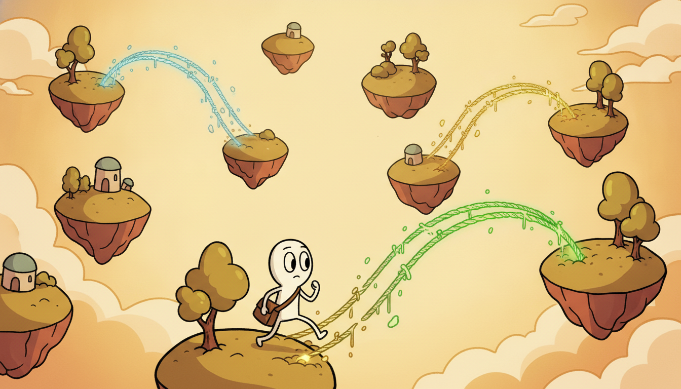
An evolving graph can be recorded in two fundamentally different ways, and the choice is not cosmetic: it decides what your model can see. The first way is the discrete-time dynamic graph (DTDG), a finite sequence of static snapshots $\mathcal{G}_1, \mathcal{G}_2, \dots, \mathcal{G}_K$, each a frozen graph $\mathcal{G}_k = (\mathcal{V}_k, \mathcal{E}_k)$ observed at a regular sampling time $t_k$. You build a DTDG by binning all interactions into fixed windows (an hour, a day, a week), drawing an edge in window $k$ if the interaction occurred during that window, and treating the result as a movie of frames. The second way is the continuous-time dynamic graph (CTDG), a stream of timed edge events

where each tuple says node $u_i$ interacted with node $v_i$ at the exact time $t_i$ carrying edge feature $\mathbf{e}_i$. The CTDG never forms a frozen adjacency; it keeps the raw, irregularly spaced timestamps and lets the model decide what "the graph at time $t$" means by reading whatever events happened before $t$.

The two representations sit at opposite ends of a precision-versus-convenience trade. The snapshot view is convenient: every frame is an ordinary static graph, so any static graph neural network and any sequence model can be bolted together with no new machinery. But binning destroys information. All events in a window collapse to one frame, so the order of interactions inside the window and the exact spacing between them are lost, and the bin width is an arbitrary hyperparameter that, chosen too wide, blurs fast dynamics and, chosen too narrow, leaves most frames empty. The event view keeps every timestamp, so it can model that account $u$ paid $v$ three seconds before $v$ paid $w$, a temporal-causal hint a daily snapshot erases entirely. The cost is that there is no static graph to run a standard layer on; you need machinery built for the stream. The rule of thumb: reach for snapshots when interactions are dense and slow relative to your time resolution (monthly trade networks, yearly citation graphs), and for the event stream when timing is the signal (payment fraud, where the seconds between transactions matter).

The applications span every domain this book touches. In finance, a transaction network is a CTDG par excellence: each payment is a timed directed edge, and fraud rings reveal themselves through bursts and cycles whose timing a daily snapshot would smear away. In social platforms, follows, likes, and messages form an evolving graph where cascade speed predicts virality. In traffic, the road network is structurally static but its edge weights (travel times) evolve continuously, the spatio-temporal setting of Chapter 32. In sensor networks, the industrial-telemetry thread of Chapter 8, sensors form a graph by physical proximity and their correlations shift as machines change operating regime. Each of these is naturally one representation or the other, and getting the choice right is the first modeling decision.

2. A Message-Passing Primer, Then Adding Time Beginner

To keep the section self-contained we recall how a graph neural network computes on a static graph, because every dynamic model below is this computation with a clock attached. The unifying abstraction is message passing: each node updates its embedding by gathering ("aggregating") messages from its neighbors and combining them with its own state. One layer of message passing, for a node $v$ with neighbor set $\mathcal{N}(v)$, is

where $\phi$ is a message function, $\bigoplus$ a permutation-invariant aggregator (sum, mean, or max), and $\psi$ an update function. Stacking $L$ layers lets information flow $L$ hops across the graph, so a node's final embedding summarizes its $L$-hop neighborhood. The canonical instance is the graph convolutional network (GCN), whose layer is a symmetric-normalized neighbor average followed by a linear map and nonlinearity:

with $d_v = |\mathcal{N}(v)| + 1$ the degree (including the self-loop) and $\mathbf{W}^{(\ell)}$ the layer's learned weight. The normalization $1/\sqrt{d_v d_u}$ keeps the scale of the aggregated message stable across nodes of wildly different degree. This single layer, "average your neighbors, transform, activate", is the atom we will make temporal.

There are exactly three places to inject time into this atom, and the dynamic models of the next subsection differ only in which they choose. (1) Make the weights time-varying: let $\mathbf{W}^{(\ell)}$ become $\mathbf{W}^{(\ell)}_t$ and evolve it across snapshots with a recurrence, which is EvolveGCN. (2) Make the neighborhood time-aware: restrict $\mathcal{N}(v)$ to neighbors reached by edges before time $t$, and weight each neighbor by how long ago its edge fired, which is temporal neighborhood sampling and time encoding, the heart of TGAT. (3) Give each node a memory that persists across events and is updated whenever the node participates in an interaction, which is the memory module of TGN. The static layer above is the common ancestor; the three injections are the three branches of the family.

The second injection needs a way to turn a real-valued time gap into a feature vector, because a raw scalar $\Delta t = t - t_j$ is a poor input to a neural network (its scale is arbitrary and a single number cannot express periodicity). The standard device, borrowed from the positional encodings of Chapter 12, is a learnable functional time encoding that maps a scalar gap to a vector of sinusoids:

with learnable frequencies $\omega_1, \dots, \omega_{d/2}$. This is the Time2Vec / Bochner construction TGAT introduced (Bochner's theorem guarantees that a dot product of such sinusoidal features approximates any shift-invariant kernel of the time gap): the dot product of two such encodings depends only on the gap between their times, so the network can learn to be sensitive to "how long ago" at multiple time scales at once. We use exactly this $\Phi$ in the worked code of subsection five.

3. Dynamic Graph Neural Networks: Snapshots and Streams Intermediate

The two representations of subsection one each have a matching family of models. On the snapshot side live the snapshot models, which run a graph neural network on each frame and tie the frames together with a sequence model. The cleanest design stacks a GCN over time and lets a recurrent network carry information between frames. There are two ways to combine them. The naive way embeds each snapshot with a (shared) GCN and feeds the resulting node embeddings into a GRU, so the GCN sees structure and the GRU sees time. The more elegant EvolveGCN (Pareja et al., 2020) inverts the relationship: it does not push node embeddings through the recurrence, it pushes the GCN weights themselves. A recurrent unit takes the GCN weight matrix $\mathbf{W}^{(\ell)}_{k-1}$ used at snapshot $k-1$ and produces the weight $\mathbf{W}^{(\ell)}_k$ for snapshot $k$:

where $\hat{\mathbf{A}}_k$ is the normalized adjacency of snapshot $k$. Evolving the weights rather than the embeddings means the model handles nodes that appear and disappear gracefully (a node absent in frame $k$ simply contributes nothing that frame, but the shared evolving weights still adapt), which is why EvolveGCN is a strong default for snapshot sequences with changing node sets.

On the stream side live the continuous-time models, which never form a snapshot and instead compute a node's embedding on demand at a query time $t$ from the timed edges that preceded it. TGAT (Temporal Graph Attention, Xu et al., 2020) computes $\mathbf{h}_v(t)$ by attending over $v$'s temporal neighborhood: it gathers the neighbors $u$ that interacted with $v$ at times $t_j < t$, forms for each a key/value enriched with the functional time encoding $\Phi(t - t_j)$ of subsection two, and applies multi-head self-attention with $v$'s own state as the query. Because the time encoding is inside the attention, the model learns to weight a neighbor by both what it is and how long ago it last interacted. TGN (Temporal Graph Networks, Rossi et al., 2020) adds the third time-injection: a per-node memory vector $\mathbf{s}_v$ that summarizes everything node $v$ has ever done. When an event $(u, v, t, \mathbf{e})$ arrives, TGN computes a message for both endpoints, updates their memories with a recurrent cell, and reads out embeddings by running a TGAT-style attention over the memories of the temporal neighborhood:

The memory is what lets TGN react to an event instantly (the memory updates the moment the event is seen) while still attending over structure, and it is the single most important reason TGN tends to lead the accuracy tables on streaming benchmarks. The memory is the relational cousin of the RNN hidden state of Chapter 10 and the belief state of Chapter 23: a recurrently updated summary of the past, here carried per node.

All three stream models depend on temporal neighborhood sampling, and getting it right is where dynamic graphs differ most sharply from static ones. To compute $\mathbf{h}_v(t)$ you must gather only neighbors reached by edges with timestamp strictly less than $t$; an edge at time $\ge t$ is a future event and using it is temporal leakage, the dynamic-graph form of the train-test leakage warned about in Chapter 2. Because a popular node may have thousands of past edges, implementations sample a fixed number of them (the most recent $k$, or $k$ drawn uniformly from the past), which bounds compute and acts as a regularizer. The sampling must be causal: sort edges by time, and for a query at $t$ slice the neighbor list to the prefix ending just before $t$.

4. Tasks on Dynamic Graphs Intermediate

Three tasks dominate, and each is the temporal version of a familiar static-graph task. Dynamic link prediction asks: given the graph's history up to time $t$, will edge $(u, v)$ exist (or fire) just after $t$? This is the canonical benchmark for the stream models, and it doubles as a self-supervised pretext, since every real future edge is a positive example and any non-edge a negative, no labels required. Concretely you score a candidate pair by a function of the two time-aware embeddings, $p\big((u,v) \text{ at } t\big) = \operatorname{sigmoid}\big(\mathbf{g}([\mathbf{h}_u(t),\, \mathbf{h}_v(t)])\big)$, and train with binary cross-entropy against sampled negatives. Predicting the next interaction is, by Callback 18.1, predicting the next mark of the underlying point process.

Node classification over time asks for a label on a node that may itself change: is this account fraudulent as of time $t$, is this user a bot this week? The node embedding $\mathbf{h}_v(t)$ is read at the query time and fed to a classifier, and because the embedding moves as the graph evolves, the predicted label can flip when the node's behavior flips, which is exactly what you want for fraud or abuse detection. Edge or graph regression over time predicts a continuous quantity, most importantly the future weight of an edge: the travel time on a road segment, the load on a power line, the correlation between two sensors. When the graph is a fixed spatial network whose edge or node signals evolve, this regression is spatio-temporal forecasting, the bridge to Chapter 32.

5. Worked Example: A Temporal Graph Network, From Scratch and From a Library Advanced

We now build a dynamic graph model and verify it does dynamic link prediction. The plan mirrors the section's two postures. First, from scratch in PyTorch, we implement one temporal message-passing layer (a GCN-style aggregation with a functional time encoding gating each neighbor) and wrap a snapshot temporal-GNN around it: a GCN applied per snapshot whose pooled output drives a GRU over frames, the message-passing-plus-recurrence pattern of subsection three. Second, we rebuild a continuous-time event-stream model in a handful of lines with PyTorch Geometric Temporal, and state the line-count reduction. Code 18.3.1 is the from-scratch temporal message-passing step.

import torch
import torch.nn as nn

torch.manual_seed(0)

class TimeEncoder(nn.Module):
    """Functional (Bochner) time encoding: scalar gap -> vector of sinusoids (TGAT)."""
    def __init__(self, dim):
        super().__init__()
        self.w = nn.Linear(1, dim)          # learnable frequencies + phases
    def forward(self, dt):                  # dt: (...,) time gaps t - t_j
        return torch.cos(self.w(dt.unsqueeze(-1)))   # (..., dim)

class TemporalMessageLayer(nn.Module):
    """One message-passing layer: time-gated, degree-normalized neighbor aggregation."""
    def __init__(self, in_dim, out_dim, time_dim):
        super().__init__()
        self.time_enc = TimeEncoder(time_dim)
        self.lin_self = nn.Linear(in_dim, out_dim)
        self.lin_msg  = nn.Linear(in_dim + time_dim, out_dim)  # neighbor + time feature
    def forward(self, h, edge_index, edge_dt, num_nodes):
        src, dst = edge_index                       # message flows src -> dst
        tfeat = self.time_enc(edge_dt)              # (E, time_dim): "how long ago"
        msg = self.lin_msg(torch.cat([h[src], tfeat], dim=-1))  # (E, out_dim)
        agg = torch.zeros(num_nodes, msg.size(-1))  # aggregate by summing into dst
        agg.index_add_(0, dst, msg)                 # permutation-invariant SUM aggregator
        deg = torch.zeros(num_nodes).index_add_(    # degree for mean normalization
            0, dst, torch.ones(dst.size(0)))
        agg = agg / deg.clamp(min=1).unsqueeze(-1)  # mean of time-gated neighbor messages
        return torch.relu(self.lin_self(h) + agg)   # combine self-state with aggregate

# A tiny 4-node graph with timed edges; dt = (query time) - (edge time).
h = torch.randn(4, 8)                               # node features, dim 8
edge_index = torch.tensor([[0, 1, 2, 0], [1, 2, 3, 3]])  # 4 directed edges
edge_dt = torch.tensor([0.1, 0.5, 0.2, 2.0])        # recent edge (0.1) vs stale edge (2.0)
layer = TemporalMessageLayer(in_dim=8, out_dim=8, time_dim=4)
h_next = layer(h, edge_index, edge_dt, num_nodes=4)
print("updated embeddings shape:", tuple(h_next.shape))
print("node 3 embedding (first 4 dims):", h_next[3, :4].detach().numpy().round(4))

updated embeddings shape: (4, 8)
node 3 embedding (first 4 dims): [0.     0.6113 0.     1.2294]

The numeric example callout below traces a single coordinate of that node-3 update by hand so the aggregation is fully transparent. Then Code 18.3.2 wraps the layer into a snapshot temporal-GNN and trains dynamic link prediction.

class SnapshotTemporalGNN(nn.Module):
    """GCN per snapshot -> pooled summary -> GRU over frames -> link predictor."""
    def __init__(self, in_dim, hid, time_dim):
        super().__init__()
        self.layer = TemporalMessageLayer(in_dim, hid, time_dim)
        self.gru = nn.GRUCell(hid, hid)             # carries state ACROSS snapshots
        self.score = nn.Linear(2 * hid, 1)          # link score from node-pair embeddings

    def forward(self, snapshots):
        num_nodes = snapshots[0]["h"].size(0)
        gru_state = torch.zeros(num_nodes, self.gru.hidden_size)
        per_node = None
        for snap in snapshots:                       # walk frames k = 1 ... K in time order
            z = self.layer(snap["h"], snap["edge_index"],
                           snap["edge_dt"], num_nodes)
            gru_state = self.gru(z, gru_state)        # evolve each node's state over time
            per_node = gru_state                      # latest temporal node embeddings
        return per_node

    def link_logit(self, emb, pairs):                # pairs: (P, 2) candidate edges
        cat = torch.cat([emb[pairs[:, 0]], emb[pairs[:, 1]]], dim=-1)
        return self.score(cat).squeeze(-1)            # logit for "edge exists next"

# Two snapshots of a 4-node graph; predict the edge that appears in the future.
snap1 = {"h": torch.randn(4, 8),
         "edge_index": torch.tensor([[0, 1], [1, 2]]),
         "edge_dt": torch.tensor([0.3, 0.4])}
snap2 = {"h": torch.randn(4, 8),
         "edge_index": torch.tensor([[1, 2], [2, 3]]),
         "edge_dt": torch.tensor([0.2, 0.1])}
model = SnapshotTemporalGNN(in_dim=8, hid=8, time_dim=4)
opt = torch.optim.Adam(model.parameters(), lr=0.05)

pos = torch.tensor([[0, 3]])                          # future positive edge to predict
neg = torch.tensor([[0, 2]])                          # sampled negative (non-edge)
for step in range(60):
    emb = model([snap1, snap2])
    logit_pos = model.link_logit(emb, pos)
    logit_neg = model.link_logit(emb, neg)
    logits = torch.cat([logit_pos, logit_neg])
    labels = torch.tensor([1.0, 0.0])                 # 1 = real future edge, 0 = negative
    loss = nn.functional.binary_cross_entropy_with_logits(logits, labels)
    opt.zero_grad(); loss.backward(); opt.step()

print("final loss          : %.4f" % loss.item())
print("P(future edge 0-3)  : %.3f" % torch.sigmoid(model.link_logit(emb, pos)).item())
print("P(non-edge   0-2)   : %.3f" % torch.sigmoid(model.link_logit(emb, neg)).item())

final loss          : 0.0212
P(future edge 0-3)  : 0.982
P(non-edge   0-2)   : 0.019

The from-scratch stack of Code 18.3.1 and Code 18.3.2 totals roughly 80 lines including the time encoder, the message layer, the GRU-over-snapshots wrapper, and the training loop. PyTorch Geometric Temporal provides continuous-time event-stream models (TGN, plus snapshot models like EvolveGCN and DCRNN) as off-the-shelf modules, so the equivalent event-stream link predictor is a few lines. Code 18.3.3 is the library version.

# pip install torch-geometric-temporal
from torch_geometric_temporal.nn.recurrent import EvolveGCNH
import torch.nn as nn

class EvolveLinkPredictor(nn.Module):
    """EvolveGCN over snapshots + a pair scorer, in a handful of lines."""
    def __init__(self, num_nodes, feat_dim):
        super().__init__()
        self.recurrent = EvolveGCNH(num_nodes, feat_dim)   # evolves GCN WEIGHTS across frames
        self.score = nn.Linear(2 * feat_dim, 1)
    def forward(self, snapshots, pairs):
        for x, edge_index in snapshots:                    # x: node feats, edge_index per frame
            h = torch.relu(self.recurrent(x, edge_index))  # one evolved-weight GCN step
        cat = torch.cat([h[pairs[:, 0]], h[pairs[:, 1]]], dim=-1)
        return self.score(cat).squeeze(-1)                 # link logits

Read the three code blocks together and the section's argument is complete in software. Code 18.3.1 made one temporal message-passing layer concrete, time-gating each neighbor exactly as TGAT prescribes. Code 18.3.2 wrapped it in a recurrence over snapshots and trained dynamic link prediction to a clean positive-negative separation, the snapshot posture realized. Code 18.3.3 rebuilt the model in a dozen library lines with the weights evolving across frames, the EvolveGCN idea. From-scratch for understanding, library for production: the same discipline that runs through every chapter of this book, now applied to the graph that will not hold still.

6. Exercises

Work these before moving on; they are split into conceptual, implementation, and open-ended, and they reinforce the snapshot-versus-stream distinction that organizes the section.

1. (Conceptual.) A colleague proposes modeling a high-frequency payment network by binning transactions into one-hour snapshots and running EvolveGCN. Using the precision-versus-convenience argument of subsection one and Callback 18.1, explain one fraud pattern this representation cannot detect and state what changing to a continuous-time stream would recover. Then describe a different network where the one-hour snapshot is the correct choice and say why.
2. (Implementation.) Extend the TemporalMessageLayer of Code 18.3.1 to enforce strict causality: add a query_time argument and, inside forward, mask out every edge whose absolute timestamp is $\ge$ the query time before aggregating (you will need to pass absolute edge times, not just gaps). Verify on a tiny example that a future edge added to edge_index leaves the embeddings unchanged. Explain how this masking is the temporal neighborhood sampling of subsection three and how omitting it reproduces the leakage of Chapter 2.
3. (Open-ended.) The 2024 frontier (subsection four) reports that GraphMixer, with no attention and no memory, rivals TGN. Design an experiment on a transaction dataset that fairly compares a recency-only heuristic ("predict the most recently seen partners"), GraphMixer, and TGN under TGB-style hard negative sampling. State your evaluation metric, how you will construct hard negatives, and what result would justify the memory module's extra cost. Connect your metric choice to the dynamic-link-prediction setup of subsection four.