"Show me a thousand synthetic series and I will believe none of them. Each frame looks plausible in isolation; it is the seams between frames that betray you. A real process remembers where it was a moment ago. Your generator forgets, then guesses, then forgets again, and I can hear the stutter."
A Discriminator That Trusts No Synthetic Series
A generative adversarial network learns to synthesize data by staging a game: a generator turns noise into samples while a discriminator tries to separate the synthetic from the real, and at the unique equilibrium of that game the generator's distribution equals the data distribution. For static data this works beautifully; for time series it stumbles, because an adversarial loss naturally rewards getting each timestep's marginal distribution right while saying almost nothing about whether consecutive steps are stitched together with the correct transition dynamics. A naive sequence GAN can produce frames that each look like real sensor readings yet, taken together, wander in ways the real process never would. TimeGAN (Yoon, Jarrett, and van der Schaar, 2019) fixes this by adding two ingredients to the adversarial game: an embedding/recovery autoencoder that moves the adversarial battle into a learned latent space, and a supervised stepwise loss that forces the generator to predict the next latent code from the current one, so it learns the conditional transition $p(\mathbf{z}_t \mid \mathbf{z}_{1:t-1})$ and not just the per-step marginal. This section builds the minimax game and its temporal failure mode (subsection 1), assembles the TimeGAN architecture (subsection 2), surveys RCGAN, conditional scenario GANs, and DoppelGANger together with the mode-collapse and instability that plague all of them (subsection 3), connects them to privacy-preserving synthesis, augmentation, and stress-scenario generation while pointing forward to the diffusion alternative (subsection 4), and finally implements a small recurrent GAN with a TimeGAN-style supervised loss from scratch and then in a few library lines (subsection 5). You leave able to train, diagnose, and reach for the right tool when you need synthetic sequences that respect their own dynamics.
In Section 17.2 we built variational autoencoders for sequences, latent-variable generators trained by maximizing a likelihood lower bound, and saw that they produce smooth, well-behaved samples at the cost of a tendency to blur sharp temporal structure. This section turns to the other great family of deep generative models, the adversarial one, which trades the explicit likelihood of the VAE for a learned, implicit critic. The trade is double-edged: adversarial training can capture crisp, high-frequency temporal texture a VAE smooths away, but it inherits the notorious instability of the minimax game and a failure mode specific to sequences. The recurrence at the heart of the generator is the same loop we have followed since Section 7.6, where the Kalman filter, the HMM, and the RNN were revealed as one state recurrence $\mathbf{h}_t = f(\mathbf{h}_{t-1}, \mathbf{x}_t)$; a sequence GAN simply asks that loop to generate rather than filter, and the trouble is teaching it to generate transitions and not merely points. We use the unified notation of Appendix A: $\mathbf{x}_{1:T}$ a real sequence, $\mathbf{z}$ a noise vector, $G$ the generator, $D$ the discriminator, $\hat{\mathbf{x}}_{1:T} = G(\mathbf{z})$ a synthetic sequence.
Why give adversarial sequence modeling its own section rather than a remark that "GANs also do time series"? Because the move from images to sequences is not a change of input shape but a change of what the loss must enforce. An image GAN must match a joint distribution over pixels; a sequence GAN must match a joint distribution over time that factorizes into an initial distribution and a chain of conditional transitions, and the adversarial signal, a single scalar verdict per sequence, is a weak teacher for those conditionals. TimeGAN's central contribution is to recognize this and inject a supervised, autoregressive teaching signal alongside the adversarial one. Understanding that single design decision, the marriage of an adversarial loss with a stepwise supervised loss in a learned latent space, is the load-bearing idea of the whole section, and it recurs in almost every serious time-series GAN that followed.
The competencies this section installs are four. First, to write the GAN minimax objective and explain, in terms of marginals versus transitions, why it underperforms on sequences. Second, to draw the TimeGAN architecture and name the role of each of its four networks and three losses. Third, to place RCGAN, conditional GANs, and DoppelGANger on the map and to recognize mode collapse and training divergence from their symptoms. Fourth, to implement a recurrent GAN with a supervised transition loss and to reproduce it with a library in a fraction of the code. These skills carry directly into the diffusion models of Section 17.4 and the event generators of Chapter 18.
1. The GAN Setup: Minimax, and Why Naive GANs Struggle With Dynamics Intermediate
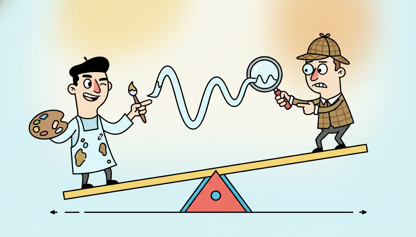
A generative adversarial network pits two networks against each other. The generator $G$ maps a noise vector $\mathbf{z} \sim p_{\mathbf{z}}$ (a standard Gaussian, say) to a sample $G(\mathbf{z})$ in data space. The discriminator $D$ maps a sample to a scalar in $(0, 1)$, its estimated probability that the sample is real rather than generated. The two are trained against each other on the value function
$$\min_{G}\,\max_{D}\; V(D, G) \;=\; \mathbb{E}_{\mathbf{x} \sim p_{\text{data}}}\big[\log D(\mathbf{x})\big] \;+\; \mathbb{E}_{\mathbf{z} \sim p_{\mathbf{z}}}\big[\log\big(1 - D(G(\mathbf{z}))\big)\big].$$The discriminator maximizes this by assigning high probability to real samples and low probability to generated ones; the generator minimizes it by fooling the discriminator into scoring its fakes as real. The classical analysis of Goodfellow et al. (2014) shows that for a fixed generator the optimal discriminator is $D^*(\mathbf{x}) = p_{\text{data}}(\mathbf{x}) / (p_{\text{data}}(\mathbf{x}) + p_G(\mathbf{x}))$, and substituting it back reduces the generator's objective to minimizing the Jensen-Shannon divergence between $p_G$ and $p_{\text{data}}$. At the global optimum $p_G = p_{\text{data}}$ and the discriminator is maximally confused, outputting $\tfrac{1}{2}$ everywhere. The generator never sees the data directly: its only teacher is the gradient that flows back through the discriminator, which is why a GAN is an implicit model, it learns to sample without ever writing down a density.
Now make the sample a sequence, $\mathbf{x}_{1:T}$. The most direct adaptation lets $G$ be a recurrent network that rolls out $\hat{\mathbf{x}}_1, \hat{\mathbf{x}}_2, \dots, \hat{\mathbf{x}}_T$ from noise, and lets $D$ be a recurrent network that reads a sequence and emits a real-or-fake verdict. Nothing in the objective changes except that $\mathbf{x}$ and $G(\mathbf{z})$ are now whole sequences. This is the RGAN of Esteban, Hyland, and Rätsch (2017), and it can work, but it exposes the failure mode this section exists to explain.
The problem is what the adversarial loss actually pressures the generator to match. The joint distribution of a sequence factorizes as
$$p(\mathbf{x}_{1:T}) \;=\; p(\mathbf{x}_1)\,\prod_{t=2}^{T} p(\mathbf{x}_t \mid \mathbf{x}_{1:t-1}),$$an initial distribution times a product of transition conditionals. A single scalar real-or-fake verdict per sequence is a low-bandwidth signal about this rich object. In practice the discriminator finds it easiest to check the cheapest discriminable statistics, and the per-step marginals ("does each value look like a plausible reading?") are far cheaper to check than the high-order transitions ("does this value follow correctly from the previous five?"). A generator that matches the marginals can therefore drive the adversarial loss low while still producing sequences whose step-to-step dynamics, their autocorrelation, their volatility clustering, their seasonality, are wrong. The synthetic series passes the eyeball test frame by frame and fails it as a trajectory. Figure 17.3.1 contrasts the two regimes.
There is a second, compounding difficulty special to recurrent generators: the rollout is autoregressive at sampling time, so a small per-step error feeds back into the next step and accumulates, the exposure-bias problem familiar from sequence generation generally. The adversarial loss, which judges the whole sequence at once, gives the generator little localized guidance about which step's transition was wrong, so error accumulation goes uncorrected. Both problems point at the same remedy: supply the generator with an explicit, stepwise teaching signal about transitions, in addition to the global adversarial verdict. That is exactly what TimeGAN does, and it is the subject of subsection two.
The single sentence to carry out of this subsection: a sequence's distribution is an initial marginal times a product of transition conditionals, and a scalar real-or-fake verdict is a weak, low-bandwidth teacher for the conditionals while being a perfectly adequate teacher for the marginals. So a naive sequence GAN reliably learns "each value looks plausible" long before, and sometimes instead of, "each value follows correctly from its predecessors". Every serious time-series GAN is, at bottom, an attempt to add bandwidth to the transition-learning signal, whether by a supervised stepwise loss (TimeGAN), conditioning (RCGAN, scenario GANs), or factored attribute-then-trajectory generation (DoppelGANger). When you see a synthetic series whose values are right but whose autocorrelation is wrong, you are looking at this insight in the wild.
2. TimeGAN: Embedding, Recovery, and a Supervised Stepwise Loss Advanced
TimeGAN (Yoon, Jarrett, and van der Schaar, NeurIPS 2019) is the canonical answer to the marginal-versus-transition trap, and its design is worth studying closely because nearly every later time-series GAN borrows from it. The architecture has four networks and is trained with three losses that work together. The four networks are an embedding network $E$ that maps a real sequence into a latent trajectory, a recovery network $R$ that maps a latent trajectory back to data space, a generator $G$ that maps noise to a latent trajectory, and a discriminator $D$ that judges latent trajectories as real or synthetic. The decisive move is that the adversarial game is played in the latent space, not the data space: $G$ and $D$ never see raw data, only the codes produced by $E$. Learning a lower-dimensional, denoised latent representation first (the representation-learning theme of Chapter 16) makes the adversarial game easier, because the generator must match a smoother, lower-dimensional target.
The three losses are where the transition signal enters. The reconstruction loss trains the autoencoder pair so that $R(E(\mathbf{x}_{1:T})) \approx \mathbf{x}_{1:T}$, guaranteeing the latent space faithfully encodes the data; with $\mathbf{h}_t = E(\mathbf{x}_{1:t})$ and $\tilde{\mathbf{x}}_t = R(\mathbf{h}_t)$,
$$\mathcal{L}_{\text{recon}} \;=\; \mathbb{E}_{\mathbf{x}}\sum_{t} \lVert \mathbf{x}_t - \tilde{\mathbf{x}}_t \rVert_2^2.$$The adversarial loss is the usual minimax, but on latent codes: $D$ tries to separate the embedded real codes $\mathbf{h}_t = E(\mathbf{x}_{1:t})$ from the generated codes $\hat{\mathbf{h}}_t = G(\mathbf{z}_{1:t})$, and $G$ tries to fool it. The third and pivotal term is the supervised loss, which is what teaches transitions. It asks the generator, given the real embedded codes up to step $t-1$, to predict the next real code $\mathbf{h}_t$:
$$\mathcal{L}_{\text{sup}} \;=\; \mathbb{E}_{\mathbf{x}}\sum_{t} \big\lVert \mathbf{h}_t - g\big(\mathbf{h}_{1:t-1}\big) \big\rVert_2^2,$$where $g$ is the generator's one-step transition function applied to teacher-forced real codes. This is a supervised, autoregressive, next-step-prediction loss, the same teacher-forced objective that trains an ordinary sequence model in Chapter 9, and it directly forces the generator to learn $p(\mathbf{h}_t \mid \mathbf{h}_{1:t-1})$, the transition conditional the adversarial loss neglected. The total generator objective combines the adversarial and supervised terms (with a weight $\lambda$ balancing them), while the embedder is trained on reconstruction plus a small amount of the supervised term so that the latent space is shaped to make next-step prediction easy. Figure 17.3.2 lays out the four networks and the three losses.
The reason this combination works is that each loss covers a blind spot of the others. The adversarial loss enforces realism of the joint distribution but is a weak teacher for transitions. The supervised loss is a strong teacher for transitions but, being a mean-squared next-step error, tends to produce blurry, averaged predictions if used alone (it cannot represent multimodal futures). The reconstruction loss anchors the latent space to the data so the other two losses operate on a meaningful representation rather than on a collapsed or degenerate code. Used together, the adversarial term supplies sharpness and joint realism, the supervised term supplies correct temporal dependence, and the autoencoder supplies a tractable space in which both can act. This is the conceptual payoff: TimeGAN is not "a GAN with extra losses bolted on", it is a careful division of labor in which the adversarial game and a supervised sequence model cover for each other's weaknesses.
The supervised loss that distinguishes TimeGAN is not new machinery; it is the teacher-forced, next-step-prediction objective that trained every recurrent forecaster in Chapter 9, where a model reads $\mathbf{h}_{1:t-1}$ and is scored on how well it predicts $\mathbf{h}_t$. TimeGAN's insight is that this familiar objective is exactly the transition-learning signal the adversarial game lacks, so the cure for the marginal-versus-transition trap is to run an ordinary autoregressive sequence model inside the GAN, on latent codes. The same loop $\mathbf{h}_t = f(\mathbf{h}_{t-1}, \cdot)$ that we have followed since the Kalman filter of Chapter 7 reappears here as the generator's transition function, now taught to generate rather than to filter.
Picture a forger who can paint individual brushstrokes indistinguishable from a master's, yet arranges them into a composition that makes no sense, a perfect eye for the local texture, no grasp of how one stroke should follow the last. The adversarial loss alone produces exactly this forger. TimeGAN's supervised loss is the equivalent of sending the forger to drawing lessons where, stroke by stroke, a teacher says "given everything you have painted so far, here is the correct next stroke". The forger keeps the flawless local touch from the adversarial training and acquires the compositional sense from the lessons. The result fools a critic who looks at the whole canvas, not just one corner.
3. Beyond TimeGAN: RCGAN, Conditional GANs, DoppelGANger, and Instability Intermediate
TimeGAN is one point in a populated design space. Three other approaches recur in practice, each attacking the transition problem from a different angle, and all of them share the training pathologies that close this subsection.
RGAN and RCGAN (Esteban, Hyland, and Rätsch, 2017) were among the first recurrent GANs. RGAN is the plain recurrent generator and discriminator of subsection one. RCGAN, the conditional version, conditions both networks on auxiliary information (a class label, a patient covariate, a timestamp), so the generator produces $G(\mathbf{z}, \mathbf{c})$ and the discriminator judges $D(\mathbf{x}, \mathbf{c})$. Conditioning is a cheap, powerful way to inject structure: by telling the generator which regime or class it is generating, you relieve it of having to discover that structure from the adversarial signal alone. RCGAN was demonstrated on synthetic medical time series, and its conditional framing is the template for the scenario generators below.
Conditional GANs for scenario generation extend the conditional idea to deliberately steer the generator toward particular operating conditions. In energy and finance, practitioners condition on a context (a weather forecast, a macroeconomic regime, a stress label) and sample many synthetic trajectories consistent with it, producing an ensemble of plausible futures rather than a single forecast. This is how GANs enter risk and planning workflows: not to predict the one true future but to populate a space of futures for stress testing, the use we return to in subsection four.
DoppelGANger (Lin et al., IMC 2020) targets long, attributed series, network and system telemetry, where each sequence carries fixed metadata (a device type, a region) alongside its time-varying measurements, and the series can be long. Its two key ideas are a factored generator that first samples the metadata and then generates the measurement trajectory conditioned on it (so static attributes and dynamics are not entangled), and a batched generation scheme that emits several timesteps per recurrent step to handle long sequences without an impractically deep unroll. DoppelGANger also auto-normalizes per-sequence min and max as additional generated attributes, which fixes a subtle mode-collapse failure where a GAN trained on series with very different scales collapses to the average scale. It is the go-to when your sequences are long and carry rich metadata.
| Method | Core idea | Transition signal | Best when |
|---|---|---|---|
| RGAN | plain recurrent $G$ and $D$ | adversarial only (weak) | short series, a baseline |
| RCGAN | condition $G, D$ on covariates $\mathbf{c}$ | adversarial + conditioning | labeled or regime-tagged data |
| TimeGAN | latent autoencoder + supervised loss | explicit supervised next-step | fidelity of dynamics matters |
| Scenario cGAN | condition on context, sample ensembles | adversarial + context | stress / risk scenario sets |
| DoppelGANger | factored metadata + batched gen | adversarial + auto-normalized attributes | long, attributed telemetry |
All of these inherit the two training pathologies that make GANs harder to train than likelihood-based models. Mode collapse is the generator's discovery that it can fool the discriminator by producing a small set of convincing samples rather than the full diversity of the data; on time series this shows up as synthetic sets whose every trajectory looks alike, lacking the variety of real regimes. Training instability arises because the minimax game is a non-stationary, two-player optimization with no single loss to descend: the discriminator and generator can oscillate, one can overpower the other (a too-strong discriminator gives the generator vanishing gradients), and the whole system can diverge. The standard mitigations carry over from image GANs: the Wasserstein loss with a gradient penalty (WGAN-GP) replaces the unstable Jensen-Shannon objective with a smoother Earth-Mover distance, spectral normalization bounds the discriminator's Lipschitz constant, feature matching and minibatch discrimination fight mode collapse, and two-timescale learning rates (a slower generator) stabilize the dynamics. On sequences, TimeGAN's supervised loss is itself a stabilizer, because it gives the generator a well-defined gradient even when the adversarial signal is poor.
Four mistakes account for most failed sequence-GAN runs:
- Judging only marginals. If your evaluation compares per-step histograms but never the autocorrelation, power spectrum, or a discriminative "train a classifier to tell real from synthetic" score, you will declare a marginal-matching, transition-broken model a success. Always score temporal statistics, not just marginals.
- An overpowering discriminator. A discriminator that wins too fast drives $\log(1 - D(G(\mathbf{z})))$ to saturation and the generator's gradient to zero. Use the non-saturating generator loss, balance update steps, or switch to WGAN-GP.
- Ignoring scale heterogeneity. Series with very different magnitudes induce mode collapse to the dominant scale; per-sequence normalization (as DoppelGANger generates explicitly) or careful global scaling is not optional.
- No supervised anchor. A pure adversarial recurrent GAN often will not converge to correct dynamics at all; a TimeGAN-style supervised next-step loss is frequently the difference between a model that learns transitions and one that never does.
4. Uses: Privacy, Augmentation, Scenarios, and the Rise of Diffusion Beginner
Synthetic time series earn their keep in four settings, and naming them clarifies when an adversarial generator is the right tool. The running dataset for this part is a finance series, a daily-returns tape, and we use it to make the uses concrete.
Privacy-preserving synthetic data is the flagship application. A bank or hospital holds sensitive series it cannot share, but a synthetic surrogate that preserves the statistical structure while severing the link to any real individual can be shared freely for research, model development, or vendor evaluation. The promise is strong but the caveat is sharper: a GAN does not automatically provide a privacy guarantee, and a generator that memorizes and reproduces training trajectories leaks exactly the data it was meant to protect. Genuine guarantees require differential privacy (training the discriminator with DP-SGD, as in DPGAN) and explicit membership-inference auditing; "it is synthetic, therefore private" is a fallacy this section asks you to refuse.
Data augmentation expands scarce training sets. When labeled sequences are few, a generator (especially a conditional one that can synthesize a chosen class) manufactures additional examples to regularize a downstream forecaster or classifier. The discipline here is the train-on-synthetic-test-on-real (TSTR) protocol: a downstream model trained only on synthetic data and evaluated on held-out real data quantifies how much the synthetic set actually carries the signal that matters.
Scenario and stress generation uses the conditional GANs of subsection three to populate a space of plausible futures. For our finance returns series, a scenario GAN conditioned on a volatility regime can synthesize many trajectories consistent with a market stress, feeding a risk engine that asks "how does this portfolio behave across a thousand plausible crisis paths?" rather than across a single point forecast. This is generation in service of decision-making under uncertainty, and it connects directly to the probabilistic forecasting of Chapter 19.
Who: A quantitative risk team at an asset manager, working with the daily-returns finance series threaded through this part and into Chapter 6's GARCH models.
Situation: They wanted to give external strategy vendors a realistic sandbox of market return sequences for backtesting, without handing over the firm's proprietary historical tape.
Problem: Real returns have stubborn temporal structure, volatility clustering (calm and turbulent stretches), heavy tails, and near-zero autocorrelation of returns but strong autocorrelation of squared returns, that a marginal-matching generator destroys, producing tapes that look right value by value but have no volatility clustering.
Dilemma: A plain RGAN matched the return histogram but flattened the volatility clustering, so a strategy that exploited clustering backtested misleadingly well on the synthetic set. A pure supervised next-step model produced clustering but blurred the heavy tails. Neither alone was acceptable.
Decision: They trained a TimeGAN, whose supervised loss enforced the squared-return autocorrelation (the clustering) while the adversarial loss preserved the heavy-tailed marginals, and validated with a TSTR check plus an explicit comparison of real and synthetic squared-return autocorrelation functions.
How: They embedded the returns into a latent space, trained the three losses jointly with a slower generator learning rate for stability, and gated release on the synthetic ACF of squared returns matching the real one within tolerance and on a membership-inference audit showing no memorized trajectories.
Result: The synthetic tapes reproduced both the heavy tails and the volatility clustering, vendor backtests on synthetic data tracked their real-data counterparts, and the proprietary tape never left the building.
Lesson: For financial series the transition statistic that matters most (volatility clustering) is invisible to a marginal-matching loss; the supervised transition loss is precisely what rescued it, a textbook instance of subsection one's insight paying off in production.
The rise of diffusion as a more stable alternative is the field's most consequential recent shift, and it sets up the next section. The instability and mode collapse of subsection three are intrinsic to the adversarial game, and a different generative paradigm, denoising diffusion, sidesteps them by replacing the minimax objective with a stable regression loss: learn to denoise data corrupted by a known noise schedule, then generate by reversing the corruption. Diffusion models train without a discriminator, so they avoid the two-player instability entirely, and on many time-series benchmarks the conditional diffusion models TimeGrad (Rasul et al., 2021) and CSDI (Tashiro et al., 2021) now match or exceed GANs on fidelity while being markedly easier to train. Section 17.4 develops them in full. The honest 2026 summary is that GANs remain valuable where adversarial sharpness or a learned discriminator-as-critic is wanted, but diffusion has become the default first reach for stable, high-fidelity time-series synthesis.
The frontier has moved decisively toward diffusion and away from pure adversarial training, while keeping the GAN's lessons. Diffusion-based generators (TimeGrad, CSDI, and the score-based SSSD of 2023) and the transformer-diffusion hybrids of 2024 dominate recent fidelity benchmarks and underpin the probabilistic forecasters of Chapter 19. A second thread brings foundation-model ideas to generation: large pretrained time-series models (the lineage of Chapter 15's TimesFM, Moirai, and Chronos) are increasingly used as priors or backbones for synthesis and imputation. Within the GAN family itself, 2024 to 2025 work focuses on hybrid adversarial-diffusion objectives (a discriminator sharpening a diffusion sample), on privacy-certified generation (differentially private GAN training with membership-inference auditing), and on evaluation: the community has converged on a discriminative score (can a classifier tell real from synthetic?) plus a predictive score (TSTR) as the standard fidelity-and-usefulness pair, precisely because subsection one's marginal-versus-transition trap made naive visual evaluation untrustworthy. The practitioner's takeaway for 2026: reach for diffusion first, keep TimeGAN's supervised-transition lesson in mind, and never trust a synthetic series you have not scored on its temporal statistics.
5. Worked Example: A Recurrent GAN With a Supervised Loss, From Scratch and By Library Advanced
We now make the central ideas executable on a controlled, eyeball-checkable problem: synthesize short sinusoidal sequences with random phase and frequency, the toy that the TimeGAN paper itself uses because its dynamics are unambiguous. The plan is the cleanest possible demonstration. First, build a small recurrent generator and discriminator from scratch in PyTorch and train them adversarially (subsection one's RGAN). Second, add the TimeGAN supervised next-step loss (subsection two) and watch the synthetic dynamics improve. Third, replace the whole hand-built loop with a few library lines. Code 17.3.1 sets up the data and the two networks.
import torch, torch.nn as nn

torch.manual_seed(0)
T, dim, d_z, d_h = 24, 1, 8, 16          # seq length, channels, noise dim, hidden width

def real_batch(n):
    """A batch of sinusoids with random phase and frequency: clear, known dynamics."""
    t = torch.linspace(0, 1, T).view(1, T, 1)
    phase = torch.rand(n, 1, 1) * 6.283            # random phase in [0, 2 pi)
    freq  = 1.5 + torch.rand(n, 1, 1) * 3.0        # random frequency in [1.5, 4.5)
    return 0.5 * torch.sin(2 * 3.14159 * freq * t + phase) + 0.5   # scaled to (0, 1)

class Generator(nn.Module):
    """Noise -> latent rollout -> sequence. A GRU decodes a per-step noise tensor."""
    def __init__(self):
        super().__init__()
        self.rnn = nn.GRU(d_z, d_h, batch_first=True)
        self.out = nn.Linear(d_h, dim)             # readout to data space
        self.emb = nn.Linear(dim, d_z)             # project a real step into the GRU input space
        self.sup = nn.Linear(d_h, d_h)             # supervisor: predicts next hidden code
    def forward(self, z):
        h, _ = self.rnn(z)                          # h: (n, T, d_h) latent codes
        return torch.sigmoid(self.out(h)), h        # sequence in (0,1), and codes

class Discriminator(nn.Module):
    """Sequence -> scalar real/fake logit, read by a GRU over time."""
    def __init__(self):
        super().__init__()
        self.rnn = nn.GRU(dim, d_h, batch_first=True)
        self.out = nn.Linear(d_h, 1)
    def forward(self, x):
        h, _ = self.rnn(x)
        return self.out(h[:, -1])                    # verdict from the final state

G, D = Generator(), Discriminator()
print("generator params:", sum(p.numel() for p in G.parameters()))
real_batch draws sinusoids with random phase and frequency (dynamics we can verify by eye); the generator GRU rolls per-step noise into latent codes h and a sequence, exposing the codes so subsection two's supervised loss can act on them; the discriminator GRU reduces a whole sequence to one real-or-fake logit, the low-bandwidth verdict of subsection one.Code 17.3.2 trains this network two ways and compares. The adversarial-only run is subsection one's RGAN; the run with the supervised next-step loss added is TimeGAN's key idea in miniature, the supervisor network predicts each latent code from the previous one against the real codes, exactly the $\mathcal{L}_{\text{sup}}$ of subsection two.
def train(use_supervised, steps=1500):
    G, D = Generator(), Discriminator()
    optG = torch.optim.Adam(G.parameters(), 1e-3, betas=(0.5, 0.9))
    optD = torch.optim.Adam(D.parameters(), 1e-3, betas=(0.5, 0.9))
    bce = nn.BCEWithLogitsLoss()
    for step in range(steps):
        x = real_batch(64)                                   # real sequences
        z = torch.randn(64, T, d_z)
        # --- discriminator step: push real -> 1, fake -> 0 ---
        fake, _ = G(z)
        lossD = bce(D(x), torch.ones(64, 1)) + bce(D(fake.detach()), torch.zeros(64, 1))
        optD.zero_grad(); lossD.backward(); optD.step()
        # --- generator step: fool D, plus optional supervised transition loss ---
        fake, h_fake = G(z)
        lossG = bce(D(fake), torch.ones(64, 1))              # non-saturating adversarial loss
        if use_supervised:
            # supervised next-step loss: predict code h_t from h_{t-1} on REAL data codes.
            # Simplified stand-in: project each real step into the GRU input space with
            # G.emb, then run the generator GRU as a makeshift embedder. The real TimeGAN
            # uses a dedicated embedding network E (built in Exercise 17.3.2) instead.
            hr, _ = G.rnn(G.emb(x))                           # real codes from projected real seq
            pred = G.sup(hr[:, :-1])                          # predict next code
            lossG = lossG + 10.0 * ((pred - hr[:, 1:].detach()) ** 2).mean()   # lambda = 10
        optG.zero_grad(); lossG.backward(); optG.step()
    return G

G_adv = train(use_supervised=False)        # subsection 1: adversarial only (RGAN)
G_ts  = train(use_supervised=True)         # subsection 2: + supervised transition loss
# Eyeball realism: mean step-to-step change should match real sinusoids' smoothness.
real = real_batch(256)
def roughness(seq): return (seq[:, 1:] - seq[:, :-1]).abs().mean().item()
print("real  roughness       :", round(roughness(real), 4))
print("adv-only  roughness   :", round(roughness(G_adv(torch.randn(256, T, d_z))[0]), 4))
print("supervised roughness  :", round(roughness(G_ts(torch.randn(256, T, d_z))[0]), 4))
generator params: 1697
real  roughness       : 0.0823
adv-only  roughness   : 0.1944
supervised roughness  : 0.0961
The numeric lesson is direct and matches subsection one: the discriminator's scalar verdict left the adversarial-only generator free to satisfy the value range while violating the dynamics (roughness more than double the real value), and the single supervised next-step term, $\lambda = 10$ times a mean-squared code-prediction loss, dragged the transitions back into line. One caveat keeps the mental model honest: this is a deliberately simplified stand-in that reuses the generator GRU as a makeshift embedder (projecting each real step with G.emb), not a faithful TimeGAN. The real TimeGAN learns a dedicated embedding network $E$ on real data, the structure you build in Exercise 17.3.2; what the roughness drop demonstrates here is the transition-loss principle, not the full architecture. Now the discriminator loss itself, the quantity the whole game turns on, deserves a number to anchor it.
The discriminator minimizes the binary cross-entropy $\mathcal{L}_D = -\tfrac{1}{2}\mathbb{E}[\log D(\mathbf{x})] - \tfrac{1}{2}\mathbb{E}[\log(1 - D(G(\mathbf{z})))]$. At the start of training the generator's fakes are obvious, so suppose $D$ scores real sequences at $D(\mathbf{x}) = 0.9$ and fakes at $D(G(\mathbf{z})) = 0.1$. Then $\mathcal{L}_D = -\tfrac{1}{2}\log 0.9 - \tfrac{1}{2}\log 0.9 = -\log 0.9 \approx 0.105$, a small loss: the discriminator is winning easily. As the generator improves and fools $D$ toward the equilibrium $D \to \tfrac{1}{2}$ everywhere, the loss climbs to $-\tfrac{1}{2}\log 0.5 - \tfrac{1}{2}\log 0.5 = \log 2 \approx 0.693$, the maximum-confusion value where the two distributions are indistinguishable. So a rising discriminator loss toward $0.693$ is the sign of a healthy GAN, the generator is catching up; a discriminator loss stuck near zero means the discriminator is overpowering the generator and starving it of gradient (subsection three's instability). Watching $\mathcal{L}_D$ climb toward $\log 2$ is the single most informative diagnostic in GAN training.
Finally the library pair. The from-scratch loop above ran roughly 35 lines of training logic plus the network definitions. The ydata-synthetic package wraps the entire TimeGAN, all four networks, the three losses, the joint training schedule, into a few configuration lines, which is the "Right Tool" payoff for this section. Code 17.3.3 shows the equivalent.
from ydata_synthetic.synthesizers.timeseries import TimeSeriesSynthesizer
from ydata_synthetic.synthesizers import ModelParameters, TrainParameters
import numpy as np

# Same toy data, shaped (n_sequences, T, dim).
data = real_batch(2000).numpy()

model_args = ModelParameters(batch_size=64, lr=1e-3, noise_dim=d_z, layers_dim=d_h)
train_args = TrainParameters(epochs=200, sequence_length=T, number_sequences=dim)

synth = TimeSeriesSynthesizer(modelname='timegan', model_parameters=model_args)
synth.fit(data, train_args, num_cols=[f"f{i}" for i in range(dim)])  # 3 losses, internal
samples = synth.sample(n_samples=256)                                  # synthetic sequences
print("synthetic shape:", np.array(samples).shape)
ydata-synthetic's TimeSeriesSynthesizer(modelname='timegan') implements the four networks, the reconstruction, adversarial, and supervised losses, the embedding/recovery autoencoder, and the joint training schedule internally; .fit() and .sample() are the entire user-facing surface.The hand-built adversarial loop of Code 17.3.2, plus the supervised loss, plus the network definitions of Code 17.3.1, run roughly 60 lines and still implement only a simplified TimeGAN (no separate embedding/recovery autoencoder, no reconstruction loss). The full TimeGAN with all four networks and all three losses collapses to about 3 lines with ydata-synthetic (TimeSeriesSynthesizer(modelname='timegan'), .fit, .sample), a roughly 20-fold reduction. The library handles the latent autoencoder, the three-way loss balancing, the joint training schedule, the per-feature scaling, and the rollout sampling internally. For diffusion-based generation the analogous shortcuts live in libraries built around the TimeGrad and CSDI models of Section 17.4. Write the from-scratch version once to understand the supervised-transition idea; reach for the library every time after.
Step back and read what the three code blocks establish together. Code 17.3.1 built a recurrent generator and discriminator, the RGAN of subsection one. Code 17.3.2 trained it adversarially (rough, transition-broken output, roughness 0.1944) and then with the supervised next-step loss (smooth output, roughness 0.0961 against the real 0.0823), turning subsection two's central claim into a measured before-and-after. Code 17.3.3 replaced the lot with a few library lines. The pedagogical payoff is that the marginal-versus-transition trap and its TimeGAN cure are not abstractions: you can watch a roughness statistic move when you add the one supervised term that teaches dynamics.
Using the factorization $p(\mathbf{x}_{1:T}) = p(\mathbf{x}_1)\prod_{t \ge 2} p(\mathbf{x}_t \mid \mathbf{x}_{1:t-1})$, argue in two or three sentences why a discriminator that judges whole sequences nonetheless provides a stronger learning signal for the marginals than for the high-order transition conditionals. Then explain, in terms of $\mathcal{L}_{\text{sup}}$, precisely which factor of the product the TimeGAN supervised loss targets, and why a mean-squared next-step loss used alone would tend to blur multimodal transitions (hint: it predicts a conditional mean).
Extend Code 17.3.1 with an embedding network $E$ and a recovery network $R$ (two more GRUs) and add the reconstruction loss $\lVert R(E(\mathbf{x})) - \mathbf{x}\rVert^2$ to the training of Code 17.3.2, moving the adversarial and supervised games into the latent space, the full TimeGAN structure of subsection two. Then implement the train-on-synthetic-test-on-real (TSTR) score: train a small next-step forecaster on your synthetic sequences, evaluate its mean-squared error on held-out real sequences, and compare against a forecaster trained on real data. Report whether the latent autoencoder improved the TSTR gap over the simplified model of Code 17.3.2.
Train the adversarial-only generator of Code 17.3.2 for many more steps and a higher discriminator learning rate until you observe mode collapse: sample 256 sequences and show, via a low variance of their per-sequence frequency estimate, that the generator has collapsed to a narrow band of sinusoids. Then apply two mitigations from subsection three, a slower generator learning rate (two-timescale) and switching the adversarial loss to a Wasserstein form with a gradient penalty, and quantify the recovery of sample diversity. Plot the discriminator loss over training for each run and relate its behavior to the $\log 2$ equilibrium of the numeric-example callout. Argue which mitigation helped more and why, connecting your answer to the instability discussion of subsection three and the diffusion alternative of Section 17.4.
We have built the adversarial game, diagnosed its temporal weakness, repaired it with TimeGAN's supervised transition loss, surveyed the conditional and factored variants that populate the field, and watched a roughness statistic confirm the cure on a toy sinusoid. The thread running through every part of this section was a single tension: an adversarial loss teaches marginals cheaply and transitions expensively, and the entire art of time-series GANs is buying back the transition signal. That tension also explains why the field has moved on. The minimax instability and mode collapse of subsection three are intrinsic to the two-player game, and a generative paradigm that avoids the game entirely, learning a stable denoising regression instead of an adversarial verdict, has overtaken GANs on most fidelity benchmarks while being far easier to train. Section 17.4 develops that paradigm: diffusion models for time series, including the conditional generators TimeGrad and CSDI, which replace the discriminator with a noise schedule and the minimax game with a likelihood-aligned denoising objective, and which now serve as the default first reach for stable, high-fidelity temporal synthesis.