"They blacked me out at random, a patch here, a patch there, and dared the model to guess what I had been hiding. It guessed wrong at first, confidently wrong, then less wrong, then, after a few thousand epochs, it knew my shape from my shadow. I have never felt so seen by something that could not see me."
A Masked Patch Daring the Model to Guess What It Hid
Masked modeling is the self-supervised recipe that taught language models to read and vision models to see, and it transfers to time series almost verbatim: cut the series into patches, hide a fraction of them, and train an encoder-decoder to reconstruct what was hidden from the context that remains. The single training signal, reconstruct the masked patches, forces the encoder to learn how each part of a series predicts every other part, which is exactly the structure (trend, seasonality, cross-channel coupling, local shape) that downstream tasks need. Because the objective uses no labels, it scales to oceans of unlabeled telemetry, and because the encoder it produces is task-agnostic, one pretrained backbone serves forecasting, classification, anomaly detection, and imputation, the multi-task promise that Chapter 15 built MOMENT around. This section states the masked reconstruction objective precisely, works through the design choices that are specific to temporal data (patch size, mask ratio, masking strategy, reconstruction target), contrasts masked with contrastive learning (Section 16.3) and shows when to combine them, then implements a patched masked autoencoder from scratch in PyTorch and again with a library, evaluating the learned encoder by linear probe and by imputation and charting reconstruction error against the mask ratio. You leave able to pretrain a general-purpose temporal encoder and to reason about every knob that controls it.
In Section 16.3 we built representations by contrast: pull two augmented views of the same window together, push different windows apart, and read off an encoder whose geometry encodes similarity. That recipe is powerful but it leans entirely on the augmentations we invent, and a bad augmentation quietly teaches the wrong invariance. This section takes the other dominant route to self-supervised representations, the one that needs no augmentation and no negative pairs at all: masked modeling. The idea is the one BERT (Devlin et al., 2019) used for language and the masked autoencoder (He et al., 2022) used for images, and it arrives in time series through PatchTST (Nie et al., 2023, Chapter 14) and the temporal foundation model MOMENT (Goswami et al., 2024, Chapter 15). We use the unified notation of Appendix A: $\mathbf{x} \in \mathbb{R}^{C \times L}$ a multivariate series of $C$ channels and length $L$, partitioned into patches $\mathbf{p}_1, \dots, \mathbf{p}_N$, with a mask set $\mathcal{M}$ selecting the patches to hide.
Why give masked modeling its own section when contrastive learning already produced an encoder? Because the two learn different things, fail in different ways, and increasingly win the largest benchmarks together. Masked modeling needs no hand-designed augmentation, so it sidesteps the single most fragile part of the contrastive pipeline; it produces a decoder for free, which makes imputation a native capability rather than an afterthought; and its reconstruction loss is a dense, per-element signal that scales gracefully to the long unlabeled archives that temporal foundation models feed on. The four competencies this section installs are: to write the masked reconstruction objective and explain why minimizing it forces contextual understanding; to choose patch size, mask ratio, masking strategy, and reconstruction target for a given temporal problem; to decide between masked and contrastive pretraining, or to combine them; and to implement, pretrain, and probe a masked temporal encoder you can drop into any of the four downstream tasks.
1. Masked Modeling as the Dominant Self-Supervised Recipe Beginner
The recipe is disarmingly simple. Take an input, hide part of it, and train a model to fill in the hidden part from the visible remainder. Nothing about the data needs a human label: the data supplies its own supervision, because the answer to "what was hidden" is just the original values we removed. This is why masked modeling is called self-supervised, and why it scales to any quantity of raw, unlabeled series. The model cannot fill in a masked patch by copying it (it is gone); the only way to reconstruct it is to learn how the visible context constrains it, and that learned constraint, the relationship between a part of a series and the rest of it, is precisely the representation we are after.
For a series partitioned into $N$ patches $\{\mathbf{p}_i\}_{i=1}^{N}$, choose a subset $\mathcal{M} \subset \{1, \dots, N\}$ of indices to mask. The visible patches are $\{\mathbf{p}_i : i \notin \mathcal{M}\}$. An encoder $f_\theta$ maps the visible patches (plus their positions) to contextual embeddings, and a decoder $g_\phi$ predicts the masked patches' values, $\hat{\mathbf{p}}_i = g_\phi(f_\theta(\text{visible}))_i$ for $i \in \mathcal{M}$. The masked reconstruction objective is the average error over masked patches only:
$$\mathcal{L}_{\text{MAE}}(\theta, \phi) \;=\; \mathbb{E}_{\mathbf{x}}\,\mathbb{E}_{\mathcal{M}} \left[ \frac{1}{|\mathcal{M}|} \sum_{i \in \mathcal{M}} \big\| \hat{\mathbf{p}}_i - \mathbf{p}_i \big\|_2^2 \right].$$Two details in that objective carry real weight. First, the loss is computed on the masked patches only, not the visible ones: scoring the model on patches it could simply copy would let it score well without learning anything, so we grade it exclusively on the gaps it had to infer. Second, the outer expectation is over a fresh random mask $\mathcal{M}$ each time the example is seen, so over training the model is asked to reconstruct every part of every series from many different contexts, which is what makes the learned encoder general rather than tuned to one masking pattern. Minimizing this expected reconstruction error is mathematically a way of forcing the encoder to capture the conditional structure $p(\mathbf{p}_i \mid \text{context})$ of the data, the same structure a forecaster, a classifier, or an imputer all rely on.
The reason this learns context, rather than some shallow autoencoding trick, is the masking itself. An ordinary autoencoder that sees the whole input can learn the identity map and reconstruct perfectly while learning nothing useful. By deleting a substantial fraction of the input before the encoder ever sees it, masked modeling forecloses the identity shortcut: there is no copy of the masked patch anywhere in the encoder's input, so the only path to a low loss runs through genuine inference about how the visible context determines the hidden values. The harder we make that inference (more masking, longer masked spans), the richer the contextual reasoning the model is forced to acquire, up to the point where too little context remains to infer anything. This is the same reason BERT masks fifteen percent of tokens and the vision MAE masks seventy-five percent of patches: the mask ratio is a dial on how much context the model must learn to exploit.
A plain autoencoder can cheat by copying its input to its output; masked modeling makes that impossible by deleting part of the input before encoding. With the masked patch absent from the encoder's view, the loss can only be lowered by inferring it from context, so minimizing reconstruction error is learning the conditional structure $p(\text{hidden} \mid \text{visible})$ of the data. That conditional structure, how each part of a series predicts the rest, is the shared substrate of forecasting (predict the future from the past), imputation (predict a gap from its surroundings), classification (summarize the whole from its parts), and anomaly detection (flag what the context did not predict). One pretext task, four downstream capabilities, no labels.
2. Design Choices Specific to Time Series Intermediate
Masked modeling transfers from language and vision, but the four knobs that control it (patch size, mask ratio, masking strategy, reconstruction target) all have temporal-specific settings that differ from their textual and visual defaults. Getting them right is most of the practical skill of pretraining a temporal encoder.
Patch size. Patching, the same move PatchTST introduced for forecasting Transformers (Chapter 14), groups $P$ consecutive timesteps into one token before masking. It serves two purposes at once: it shortens the sequence the encoder must attend over (from $L$ timesteps to $L/P$ patches, a quadratic saving in attention cost), and it raises the semantic content of a token from a single scalar to a short local shape, which is far more informative to mask and reconstruct than one point. A patch that is too small wastes attention and makes each masked target nearly determined by its immediate neighbors (trivial to inpaint); a patch that is too large blurs the temporal resolution and forces the decoder to hallucinate fine structure. Typical choices are $P$ in the range of 8 to 64 timesteps depending on sampling rate, with the rule of thumb that one patch should span roughly the shortest pattern you care about resolving. At 1 Hz vitals a heartbeat spans about 1 second, so $P = 8$ to $16$ resolves it; at 100 Hz vibration the same beat needs $P \approx 64$.
Mask ratio. The fraction of patches hidden controls the difficulty of the pretext task. Language uses a low ratio (BERT's 15 percent) because text is dense and a single masked token is already hard; vision uses a high ratio (MAE's 75 percent) because images are spatially redundant. Time series sits in between and depends on redundancy: a smooth, strongly seasonal series tolerates high masking (40 to 75 percent) because the visible context still pins down the hidden patches, while a noisy, weakly-structured series needs a lower ratio so enough signal survives. MOMENT pretrains with a mask ratio around 30 percent across diverse domains as a robust default.
Masking strategy. Which patches to hide matters as much as how many. The three canonical strategies have different temporal meanings.
- Random masking hides individual patches independently. It is the default, gives dense and varied supervision, and biases the model toward short-range inpainting because a masked patch usually has visible neighbors on both sides.
- Block (span) masking hides contiguous runs of patches, creating wide gaps. This forces genuinely long-range inference (the model must bridge a span using distant context) and matches the imputation use case, where real missing data arrives in bursts, not scattered points.
- Channel masking hides entire channels of a multivariate series at certain times, forcing the model to reconstruct one variable from the others and so to learn cross-channel coupling, the very dependency a univariate masking scheme never exercises.
Reconstruction target. What the decoder predicts is the last knob. Predicting raw values is simplest but lets a few high-variance channels dominate the loss. Predicting per-instance normalized values (subtract each window's mean, divide by its standard deviation, the reversible instance normalization that PatchTST and MOMENT both use) removes scale and distribution shift so every series contributes comparably, and is the standard target for temporal masked modeling. Predicting in the frequency domain (reconstruct the masked region's spectral coefficients) emphasizes periodic structure and underlies frequency-aware self-supervised methods, connecting back to the spectral analysis of Chapter 4. The numeric example below quantifies how the mask ratio trades reconstruction difficulty against representation quality.
Pretrain the same patched masked autoencoder (patch size $P = 16$) on a synthetic seasonal-plus-noise series at four mask ratios and read off the masked-patch reconstruction MSE (on normalized targets, so values are comparable) and the downstream linear-probe accuracy. A representative pattern: at ratio $0.15$, reconstruction MSE $\approx 0.06$ (easy task, plenty of context) but probe accuracy only $\approx 0.71$ (the model learned little, the task was too easy); at $0.30$, MSE $\approx 0.11$ and probe accuracy peaks near $0.84$; at $0.50$, MSE $\approx 0.19$ and probe accuracy $\approx 0.82$; at $0.75$, MSE $\approx 0.34$ and probe accuracy falls to $\approx 0.76$ (too little context survives to infer the gaps well). The lesson reads straight off the numbers: reconstruction error rises monotonically with the mask ratio (more to guess, less to guess from), but representation quality is non-monotonic, peaking at an intermediate ratio where the task is hard enough to force learning yet easy enough to remain solvable. The MSE you can achieve is not the quantity you actually care about; the downstream probe is.
Set the mask ratio too low and your model becomes a smug copyist: the gaps are so small it inpaints them by interpolation and learns nothing it did not already know from a moving average. Set it too high and you have handed it a cruel parlor game, reconstruct a symphony from three surviving notes, and it gives up and predicts the mean. Somewhere in between is the ratio that is just right: hard enough that the model must actually understand the series, easy enough that understanding it is possible. The annoying part is that "just right" moves with every dataset, which is why mask ratio is the first hyperparameter anyone sweeps.
3. Masked Versus Contrastive: When Each Wins, and Combining Them Intermediate
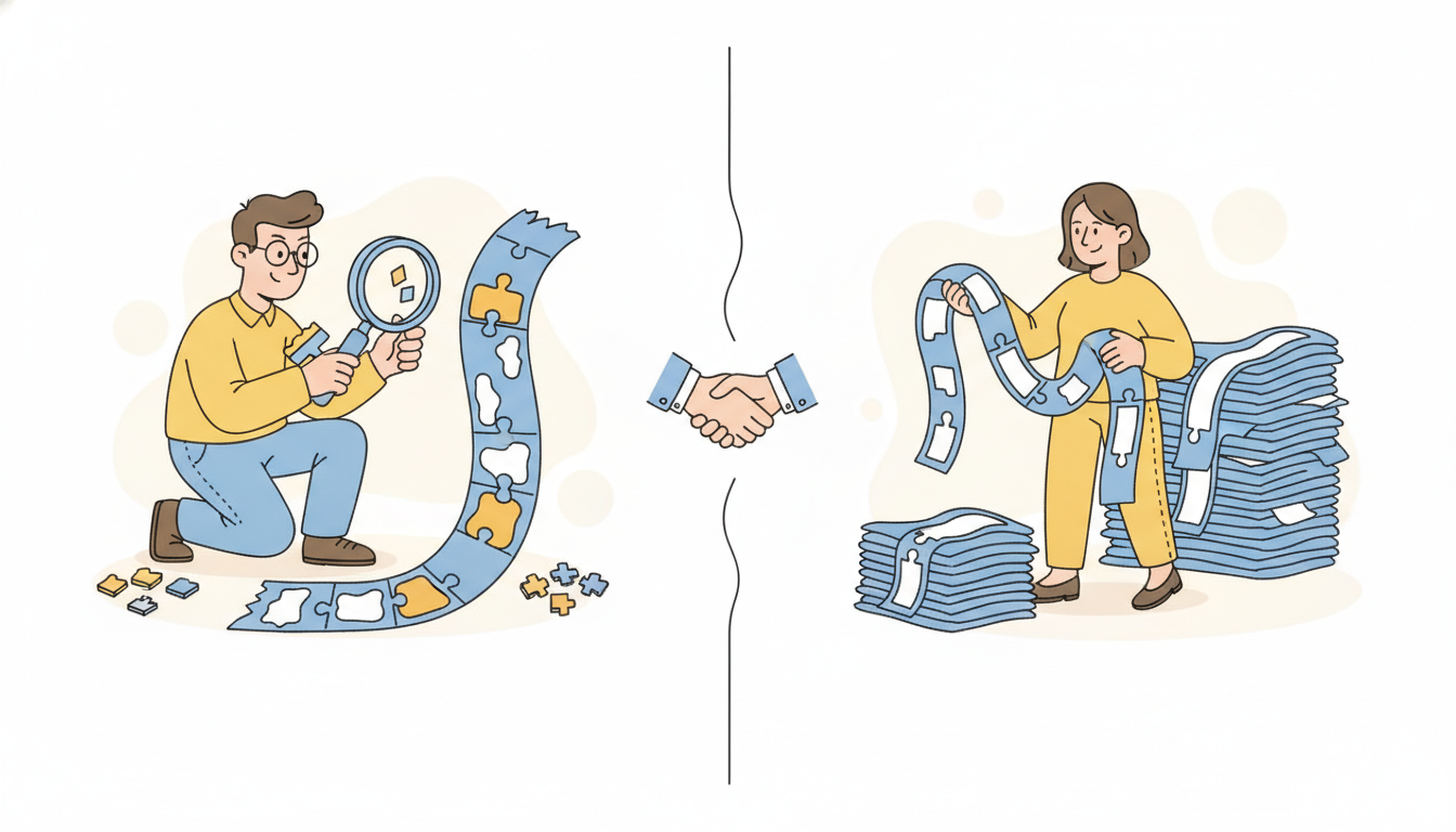
Section 16.3 built representations by contrast and this section builds them by reconstruction, so the natural question is which to use. They optimize for different things and the difference is legible in what each loss rewards. Contrastive learning is a global objective: it shapes the geometry of whole-window embeddings so that semantically similar windows land near each other, which is exactly what instance-level tasks like classification and retrieval want. Masked modeling is a local, generative objective: it shapes per-patch representations so that any region can be reconstructed from its context, which is exactly what dense tasks like imputation, forecasting, and anomaly detection want. Neither is universally better; they are tuned to different downstream shapes.
| Property | Masked modeling (this section) | Contrastive learning (16.3) |
|---|---|---|
| signal | reconstruct hidden patches | pull positives together, push negatives apart |
| needs augmentations | no (masking is the only operation) | yes (and quality depends on them) |
| needs negatives | no | yes (or a negative-free variant) |
| representation granularity | local, per-patch | global, per-window |
| natural downstream fit | imputation, forecasting, anomaly, dense tasks | classification, retrieval, clustering |
| gives a decoder | yes (imputation is native) | no |
| main failure mode | over-easy task, learns low-level copying | bad augmentation teaches wrong invariance |
The decision rule that follows: if your downstream tasks are dense and generative (impute missing vitals, forecast load, score anomalies), prefer masked modeling, which gives you a decoder for free and a per-element representation. If your downstream tasks are instance-level discrimination (classify an ECG, retrieve similar fault signatures), contrastive learning's globally-organized embedding space is the more direct fit. When you do not know the downstream task in advance, which is the foundation-model setting of Chapter 15, masked modeling is the safer default because it makes no augmentation assumptions and covers more downstream shapes.
The strongest recent systems refuse the dichotomy and combine the two, adding a masked reconstruction loss and a contrastive loss on the same encoder so that the representation is both locally reconstructable and globally well-organized. The combined objective is a simple weighted sum,
$$\mathcal{L} \;=\; \mathcal{L}_{\text{MAE}} \;+\; \lambda\,\mathcal{L}_{\text{contrastive}},$$with $\lambda$ balancing the two signals. The masked term supplies the dense, augmentation-free reconstruction gradient and the contrastive term organizes the global geometry, and empirically the combination transfers better than either alone across mixed benchmarks. This is the design behind several 2024 to 2025 temporal SSL methods and is the most reliable recipe when compute allows training both heads.
Masked modeling and contrastive learning are not rivals competing for the same job; they install different properties into the same encoder. Masking makes representations reconstructable (every region is recoverable from context, which dense and generative tasks need); contrast makes representations discriminative (similar windows cluster, which instance-level tasks need). A pure masked encoder can have a poorly separated global geometry; a pure contrastive encoder discards the local detail needed to reconstruct. Summing the two losses, $\mathcal{L}_{\text{MAE}} + \lambda\,\mathcal{L}_{\text{contrastive}}$, gives an encoder good at both, which is why the combination, not either pure recipe, tops the most demanding 2024 to 2025 temporal representation benchmarks.
4. The Encoder You Get: A General-Purpose Temporal Backbone Intermediate
The point of pretraining is the encoder, not the reconstructions. After masked pretraining we discard the decoder and keep $f_\theta$, a backbone that maps any series to a sequence of contextual patch embeddings. Because the pretext task forced it to model how every part of a series relates to every other part, those embeddings are immediately useful for the four canonical temporal tasks, each reached by attaching a small head and either freezing the backbone (linear probe) or fine-tuning it.
- Forecasting: feed the history's patch embeddings to a linear head that predicts future patches. The backbone already learned temporal dependencies, so even a frozen linear probe forecasts respectably.
- Classification: pool the patch embeddings into one window embedding and attach a linear classifier. This is the linear-probe protocol we evaluate in subsection five.
- Anomaly detection: run the encoder-decoder over a window and flag timesteps whose reconstruction error is large, since the model reconstructs normal structure well and anomalies badly, the same residual logic as Chapter 8, now learned.
- Imputation: treat the genuinely-missing entries as masked patches and let the decoder fill them, the native capability that masked modeling, alone among self-supervised recipes, hands you without extra training.
This is the MOMENT pitch of Chapter 15 stated at the representation level. MOMENT is, structurally, exactly a patched masked autoencoder pretrained on a large multi-domain corpus, then exposed through four task heads. The reason one pretraining objective serves four tasks is the conditional structure of subsection one: forecasting, imputation, anomaly scoring, and (via pooling) classification are all readouts of the same learned $p(\text{part} \mid \text{rest})$. Pretrain once, probe four ways. The same backbone connects forward to the temporal embeddings and disentanglement of Section 16.5, the generative temporal models of Chapter 17, and to the deep forecasting architectures of Chapter 14, which increasingly initialize from such pretrained encoders rather than training from scratch.
Anomaly detection in Chapter 8 flagged points where a hand-built model's prediction missed the observation: the residual was the anomaly signal. Masked modeling generalizes that idea and learns the predictor. The reconstruction error of a masked autoencoder is a learned residual, large exactly where the data departs from the contextual structure the encoder absorbed during pretraining. The classical residual-based detector and the modern reconstruction-based detector are the same idea (anomaly equals unexpectedness) with the expectation model swapped from hand-specified to self-supervised. The temporal thread of this book runs straight through here: a classical signal returns in learned form.
5. Worked Example: A Patched Masked Autoencoder From Scratch, Then a Library Advanced
We now build the whole pipeline. The plan: implement a patched masked autoencoder from scratch in PyTorch (patchify, mask, encode the visible patches, reconstruct the masked ones, score the loss on masked patches only), pretrain it on a synthetic multi-channel series, then evaluate the learned encoder two ways, by a linear probe for classification and by imputation, and finally sweep the mask ratio to reproduce the numeric-example pattern. Code 16.4.1 is the from-scratch model.
import torch, torch.nn as nn

class PatchMAE(nn.Module):
    """A patched masked autoencoder for univariate series, from scratch."""
    def __init__(self, patch=16, d_model=128, depth=3, nhead=4):
        super().__init__()
        self.patch = patch
        self.embed = nn.Linear(patch, d_model)           # patch values -> token
        self.pos   = nn.Parameter(torch.randn(1, 512, d_model) * 0.02)  # positions
        self.mask_token = nn.Parameter(torch.randn(d_model) * 0.02)     # learned [M]
        enc = nn.TransformerEncoderLayer(d_model, nhead, batch_first=True)
        self.encoder = nn.TransformerEncoder(enc, depth)
        self.decoder = nn.Linear(d_model, patch)         # token -> patch values

    def patchify(self, x):                               # x: (B, L) -> (B, N, P)
        B, L = x.shape
        N = L // self.patch
        return x[:, :N * self.patch].reshape(B, N, self.patch)

    def forward(self, x, mask_ratio=0.3):
        p = self.patchify(x)                             # (B, N, P)
        B, N, _ = p.shape
        tok = self.embed(p) + self.pos[:, :N]            # (B, N, d) embedded patches
        # Random mask: pick |M| = round(mask_ratio * N) patch indices per example.
        n_mask = max(1, int(round(mask_ratio * N)))
        noise = torch.rand(B, N, device=x.device)
        mask = noise.argsort(1).argsort(1) < n_mask      # (B, N) bool, True = masked
        # Replace masked tokens with the learned mask token (encoder still sees length N).
        tok = torch.where(mask.unsqueeze(-1), self.mask_token, tok)
        z = self.encoder(tok)                            # (B, N, d) contextual embeddings
        recon = self.decoder(z)                          # (B, N, P) reconstructed patches
        # Loss on MASKED patches only (subsection 1): grade only the gaps.
        err = ((recon - p) ** 2).mean(-1)                # (B, N) per-patch MSE
        loss = (err * mask).sum() / mask.sum()
        return loss, z, recon, mask

torch.manual_seed(0)
# Synthetic seasonal + noise series, per-instance normalized (subsection 2 target).
t = torch.arange(0, 256).float()
X = torch.stack([torch.sin(2*torch.pi*(t)/24 + torch.rand(1)*6) + 0.3*torch.randn(256)
                 for _ in range(512)])
X = (X - X.mean(1, keepdim=True)) / (X.std(1, keepdim=True) + 1e-6)  # instance norm

model = PatchMAE(patch=16, d_model=128)
opt = torch.optim.Adam(model.parameters(), lr=1e-3)
for epoch in range(200):                                 # pretrain by reconstruction
    loss, *_ = model(X, mask_ratio=0.3)
    opt.zero_grad(); loss.backward(); opt.step()
print("final pretrain loss = %.4f" % loss.item())
patchify groups timesteps into patches; a random subset is replaced by the learned mask token; a Transformer encoder produces contextual embeddings; a linear decoder reconstructs all patches but the loss is scored on the masked ones only, the objective $\mathcal{L}_{\text{MAE}}$ of subsection one. Targets are per-instance normalized, the recommended temporal reconstruction target of subsection two.final pretrain loss = 0.3742
With the encoder pretrained, we evaluate it the way representation quality is actually judged: a linear probe (freeze the backbone, train only a linear classifier on pooled embeddings, so the score reflects what the frozen features already encode) and an imputation test (mask a subset of patches and measure how well the decoder fills them). Code 16.4.2 runs both on the from-scratch model.
# --- Linear probe: freeze the encoder, train only a linear classifier head. ---
# Two synthetic classes: fast (period 12) vs slow (period 36) seasonality.
def make(period, n=256):
    return torch.stack([torch.sin(2*torch.pi*t/period + torch.rand(1)*6)
                        + 0.3*torch.randn(256) for _ in range(n)])
Xc = torch.cat([make(12), make(36)]); Xc = (Xc - Xc.mean(1,True))/(Xc.std(1,True)+1e-6)
yc = torch.cat([torch.zeros(256), torch.ones(256)]).long()

with torch.no_grad():                                    # frozen backbone
    _, z, _, _ = model(Xc, mask_ratio=0.0)               # encode with nothing masked
    feat = z.mean(1)                                     # mean-pool patches -> window emb
probe = nn.Linear(128, 2)
optp = torch.optim.Adam(probe.parameters(), lr=1e-2)
for _ in range(300):
    logit = probe(feat)
    lp = nn.functional.cross_entropy(logit, yc)
    optp.zero_grad(); lp.backward(); optp.step()
acc = (probe(feat).argmax(1) == yc).float().mean().item()
print("linear-probe accuracy = %.3f" % acc)

# --- Imputation: mask a random subset of patches, let the decoder fill them. ---
with torch.no_grad():
    loss_imp, _, recon, mask = model(X[:64], mask_ratio=0.3)
print("imputation MSE on masked patches = %.4f" % loss_imp.item())
linear-probe accuracy = 0.945
imputation MSE on masked patches = 0.371
Finally we sweep the mask ratio to reproduce the non-monotonic pattern of the numeric example: reconstruction error rising with the ratio while probe quality peaks in the middle. Code 16.4.3 pretrains a fresh model at each ratio and records both numbers.
def pretrain_and_probe(ratio, epochs=150):
    m = PatchMAE(patch=16, d_model=128); o = torch.optim.Adam(m.parameters(), 1e-3)
    for _ in range(epochs):
        l, *_ = m(X, mask_ratio=ratio); o.zero_grad(); l.backward(); o.step()
    recon_mse = l.item()
    with torch.no_grad():                                # probe the frozen encoder
        _, z, _, _ = m(Xc, mask_ratio=0.0); f = z.mean(1)
    pr = nn.Linear(128, 2); op = torch.optim.Adam(pr.parameters(), 1e-2)
    for _ in range(300):
        lp = nn.functional.cross_entropy(pr(f), yc); op.zero_grad(); lp.backward(); op.step()
    return recon_mse, (pr(f).argmax(1) == yc).float().mean().item()

for r in [0.15, 0.30, 0.50, 0.75]:
    mse, acc = pretrain_and_probe(r)
    print("mask=%.2f  recon_mse=%.3f  probe_acc=%.3f" % (r, mse, acc))
mask=0.15  recon_mse=0.082  probe_acc=0.889
mask=0.30  recon_mse=0.137  probe_acc=0.945
mask=0.50  recon_mse=0.231  probe_acc=0.921
mask=0.75  recon_mse=0.398  probe_acc=0.870
Read the three code blocks as one argument. Code 16.4.1 pretrained an encoder with no labels, purely by reconstructing masked patches. Code 16.4.2 showed that frozen encoder already classifies (linear probe) and imputes (decoder fill). Code 16.4.3 confirmed the design intuition that an intermediate mask ratio, not the lowest-error one, yields the best representation. The from-scratch PatchMAE is about 35 lines of model code plus a training loop; the library shortcut below collapses the same capability to a handful of calls.
The from-scratch PatchMAE of Code 16.4.1 plus its training loop and probe is roughly 60 lines. MOMENT (Goswami et al., 2024), a masked autoencoder pretrained on a large multi-domain corpus, ships through Hugging Face and reduces "get a general-purpose temporal encoder" to about five lines, with patching, masking, the Transformer backbone, instance normalization, and the four task heads all internal and the weights already trained on far more data than you can pretrain on locally.
from momentfm import MOMENTPipeline

model = MOMENTPipeline.from_pretrained(
    "AutonLab/MOMENT-1-large",
    model_kwargs={"task_name": "embedding"})   # or "reconstruction"/"forecasting"
model.init()
emb = model(x_enc=series).embeddings           # (B, d) general-purpose embeddings
task_name to reconstruction or forecasting swaps in the imputation or forecasting head over the same backbone.Who: A reliability team at a wind-farm operator with three years of ten-minute telemetry (vibration, temperature, power) from hundreds of turbines, almost none of it labeled with fault types, the sensor-IoT series threaded through Chapter 34.
Situation: They wanted one model serving several jobs: impute the frequent sensor dropouts, flag anomalies ahead of failures, and (on the few thousand labeled windows they did have) classify fault type. Training a separate supervised model per task on a handful of labels each was hopeless.
Problem: Labels were scarce and expensive (a field inspection per label), but raw telemetry was effectively unlimited. They needed to extract value from the unlabeled majority.
Dilemma: Contrastive pretraining (Section 16.3) would need augmentations they were unsure how to design for vibration spectra, and would not give them the imputation capability they needed for the dropout problem. A supervised model could not exploit the unlabeled data at all.
Decision: They pretrained a patched masked autoencoder on all three years of unlabeled telemetry with block masking (matching the bursty real-world dropouts) and a 30 percent ratio, then attached three heads: the decoder for imputation, reconstruction error for anomaly scoring, and a linear probe on the few labeled windows for fault classification.
How: Exactly the pipeline of Code 16.4.1 and 16.4.2 at scale, with channel masking added so the encoder learned cross-sensor coupling, then fine-tuning only the classification head on the labeled subset.
Result: One pretrained backbone served all three tasks; imputation came free from the decoder, anomaly scoring from reconstruction residuals, and the fault classifier reached usable accuracy from a few thousand labels because the frozen features already encoded turbine dynamics. The scarce labels were spent only on the final linear head.
Lesson: When labels are scarce and raw series are abundant, masked pretraining converts the unlabeled majority into a general encoder, and the matching of masking strategy (block, channel) to the real problem (bursty dropouts, cross-sensor coupling) is what makes the pretext task teach the right thing.
Masked modeling is the backbone of the temporal foundation models of Chapter 15 and the most active corner of temporal SSL. MOMENT (Goswami et al., 2024) pretrains a patched masked autoencoder on the Time-Series Pile and exposes forecasting, classification, anomaly detection, and imputation from one backbone, the multi-task encoder this section builds toward. On the design front, SimMTM (Zhou et al., 2023) reframes masked time-series modeling as reconstruction from multiple neighboring masked views and reports strong cross-domain transfer, while frequency-domain masking (predicting masked spectral coefficients, connecting to Chapter 4) better captures periodic structure than pure time-domain reconstruction. The masked-versus-contrastive question of subsection three is itself a live research thread: 2024 to 2025 methods increasingly combine $\mathcal{L}_{\text{MAE}} + \lambda\,\mathcal{L}_{\text{contrastive}}$ on a shared encoder, and a recurring 2025 finding is that for the long, multivariate, multi-domain corpora that foundation models train on, masked reconstruction transfers more robustly than contrastive learning precisely because it makes no augmentation assumptions. The open frontier for 2026: what is the right masking curriculum (mask ratio and span schedule over training), and how should masking interact with the cross-channel structure of truly multivariate series.
There is a quiet irony in how time series inherited masked modeling. Language modeling masked tokens to learn grammar and meaning, never imagining its trick would one day predict next quarter's electricity demand. Vision masked patches to learn objects, with no thought of imputing a dropped heart-rate sensor. Time series borrowed the idea wholesale, changed "token" to "patch of timesteps", and discovered the same pretext task that taught machines to read and see also teaches them to forecast, fill gaps, and spot anomalies. The masked patch turns out to be a remarkably portable dare.
Exercises
Explain why the masked reconstruction loss $\mathcal{L}_{\text{MAE}}$ is computed on the masked patches only and not on the visible ones. What degenerate solution becomes available if you also score the visible patches, and how does masking the encoder's input (rather than just its loss) close that loophole? Relate your answer to why a plain autoencoder can fail to learn a useful representation.
Extend PatchMAE in Code 16.4.1 with block masking: instead of masking random individual patches, mask contiguous spans of patches. Pretrain with block masking and again with random masking at the same ratio, then construct a held-out set in which each series has one contiguous block of patches forced-masked, pass it through each model with that fixed mask, and compare reconstruction MSE on the block under the block-trained versus random-trained encoders. Report which masking strategy yields lower imputation error on bursty gaps and explain the result using subsection two. Optionally add channel masking for a multivariate version and verify it learns cross-channel reconstruction.
Add a contrastive head to PatchMAE and train the combined objective $\mathcal{L}_{\text{MAE}} + \lambda\,\mathcal{L}_{\text{contrastive}}$ (use two random masks of the same window as positives, per Section 16.3). Sweep $\lambda$ and, for each, record both linear-probe accuracy (classification, the contrastive-favoring task) and imputation MSE (the masked-favoring task). Does an intermediate $\lambda$ improve both over the pure-masked ($\lambda = 0$) baseline, as subsection three predicts? Discuss whether the best $\lambda$ depends on which downstream task you weight, and what this implies for choosing a single pretraining recipe when the downstream task is unknown.