"They scaled me, rounded me, and looked up each of my numbers in a dictionary of five hundred bins. Now I sit in a vocabulary between token 304 and token 306, and a language model reads me left to right as though I were a sentence about the weather. I am not a sentence. I am a quarter of demand in a substation in Ohio. But I have learned to predict my own next word, so perhaps the difference no longer matters."
A Quantized Time Series Pretending to Be a Sentence
The 2024 wave of temporal foundation models took the recipe that made large language models work, pretrain one big sequence model on an enormous corpus, then deploy it zero-shot on series it has never seen, and ported it to time series by three different routes. Chronos (Amazon, 2024) takes the most literal route: scale a numeric series, quantize it into a fixed vocabulary of a few thousand bins, and train an off-the-shelf T5 language model to predict the next token, so forecasting becomes, byte for byte, language modeling, and probabilistic forecasts fall out by sampling token sequences. Lag-Llama (2024) keeps the numbers numeric but borrows the LLaMA decoder-only architecture, feeds it lag features, and outputs the parameters of a probability distribution at each step, the first open univariate time-series foundation model trained across many domains. MOMENT (2024) trains by masked reconstruction in the BERT style and ships one frozen backbone that handles forecasting, classification, anomaly detection, and imputation through lightweight task heads, the "one model, many tasks" pitch. This section explains each design, gives an honest account of where their zero-shot accuracy beats the classical baselines of Chapter 5 and where it does not, and then makes the central trick concrete: a from-scratch implementation of the scale-and-quantize tokenizer that turns a series into language-model tokens, paired with a three-line HuggingFace call that produces a zero-shot probabilistic forecast on a new series. You leave able to read the three model cards, reason about when a pretrained forecaster is the right tool, and run one yourself.
In Section 15.1 we asked what it would even mean for a time-series model to be a "foundation model": one network, pretrained once on a broad corpus of series, that transfers zero-shot or few-shot to new forecasting problems the way a pretrained language model transfers to new text tasks. That section laid out the pretraining-and-transfer paradigm in the abstract. This section makes it concrete by dissecting the three open models that defined the 2024 landscape: Chronos, Lag-Llama, and MOMENT. They are worth studying together because they stake out three genuinely different answers to the same question, "how do you pretrain a single model that forecasts any series?", and the contrasts between them teach more than any one alone. Section 15.3 continues with the commercial and multivariate frontier (TimeGPT, TimesFM, Moirai); here we build the foundations and run code.
The reason these models matter to a practitioner is a change in the default workflow. For decades the answer to "I have a new series to forecast" was "fit a model to that series": estimate an ARIMA, tune a Prophet, train a neural net on your data. A foundation model offers a different default: "call a pretrained model that has already seen millions of series, and ask it for a forecast on yours, with no fitting at all". When that zero-shot forecast is good enough, it collapses days of per-series modeling into a single API call. When it is not, you fall back to the per-series methods of Parts II and III, ideally fine-tuning the foundation model on your data rather than starting from scratch. Knowing which regime you are in, and why, is the practical payoff of this section, and the honest assessment in subsection four is where we draw that line.
The four competencies this section installs are these: to explain the Chronos pipeline of scaling, quantization, language-model training, and sampling, and to write the tokenizer yourself; to contrast that token-based design with Lag-Llama's numeric decoder-only probabilistic head and MOMENT's masked-reconstruction multi-task backbone; to state, with evidence, where zero-shot foundation forecasts beat seasonal-naive and ARIMA baselines and where they lose; and to load one of these models from HuggingFace and produce a calibrated probabilistic forecast on a series it has never seen, in a handful of lines.
1. Chronos: Forecasting as Language Modeling Intermediate
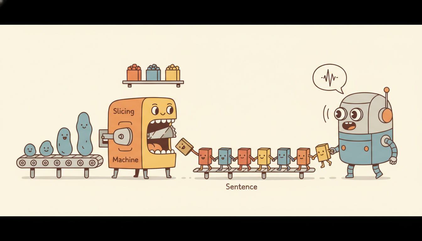
Chronos, released by Amazon Science in March 2024 (Ansari et al., "Chronos: Learning the Language of Time Series"), is built on a deliberately provocative bet: that a numeric forecasting problem can be turned, with almost no loss, into the exact text problem that language models already solve, so that the entire mature machinery of pretrained language models, the T5 architecture, the cross-entropy training objective, the sampling-based decoders, applies unchanged. The bet pays off because the only real gap between "predict the next word" and "predict the next value" is that words come from a finite vocabulary while values are continuous. Close that gap by discretizing the values, and a time series literally becomes a sentence in a small synthetic language.
The pipeline has four stages, and the first two are the entire trick:
- Scale. Divide the series by its mean absolute value, removing magnitude.
- Quantize. Map each scaled value to one of $B$ discrete bins, turning the series into integer tokens.
- Train. Fit a standard T5 language model on those tokens with next-token cross-entropy.
- Sample. Autoregressively draw token paths from the decoder, then de-quantize and un-scale into a forecast.
Scaling removes the arbitrary magnitude of a series so that a substation reading hundreds of megawatts and a stock price near forty dollars look the same to the model. Chronos uses mean scaling: divide the context window by the mean absolute value of its observations,
$$\tilde{x}_t = \frac{x_t}{s}, \qquad s = \frac{1}{C}\sum_{i=1}^{C} |x_i|,$$where $C$ is the context length and $s$ the per-series scale factor, kept aside so the forecast can be un-scaled at the end. Quantization then maps each scaled real value to one of $B$ discrete bins. With bin edges $b_0 < b_1 < \cdots < b_B$ chosen to cover the typical range of scaled values (Chronos uses $B$ on the order of four thousand, with edges spanning roughly $[-15, 15]$), the token assigned to value $\tilde{x}_t$ is the index of the bin it falls in:
$$q(\tilde{x}_t) = k \quad \text{such that} \quad b_{k-1} \le \tilde{x}_t < b_k, \qquad k \in \{1, \dots, B\}.$$The series of real numbers $x_1, \dots, x_C$ has now become a sequence of integer token ids $q(\tilde{x}_1), \dots, q(\tilde{x}_C)$, drawn from a fixed vocabulary of $B$ symbols plus a handful of special tokens (padding, end-of-sequence). That integer sequence is indistinguishable, to a language model, from a tokenized sentence. The remaining two stages are then pure language modeling. Training feeds these token sequences to a standard T5 encoder-decoder and minimizes the next-token cross-entropy, the identical objective used to pretrain T5 on text, over a large corpus of real and synthetic series. Sampling produces forecasts: to predict $H$ steps ahead, autoregressively sample $H$ tokens from the decoder, map each sampled token back to the center (or a within-bin value) of its bin, and un-scale by $s$. Drawing many such sample paths gives an empirical predictive distribution, so probabilistic forecasting is free, it is just the language model's own next-token distribution read out as quantiles.
Two design consequences are worth flagging because they shape when Chronos is the right tool. First, because the vocabulary is fixed and finite, Chronos cannot in principle produce a value outside its quantization range; a series that, after scaling, lands beyond the outermost bin edge is clipped, so Chronos is weakest on series with extreme outliers or unbounded trends that scaling does not tame. Second, because quantization throws away within-bin precision, the forecast resolution is bounded by the bin width, which is why Chronos uses thousands of bins rather than dozens. These are exactly the tradeoffs the from-scratch tokenizer in subsection five makes visible. The original release ships several sizes (Chronos-T5-tiny through -large), and a 2024 follow-up, Chronos-Bolt, restructures the model for an order-of-magnitude speedup, which matters because the autoregressive token-by-token decoding of the original is its main latency cost.
The conceptual leap in Chronos is not the T5 model, which is borrowed unchanged, but the realization that the only thing separating numeric forecasting from text modeling is the continuous-versus-discrete gap, and that quantization closes it. Once a value is a token, every tool built for language, pretraining at scale, cross-entropy, sampling, beam search, temperature, transfers for free. The cost is the two losses quantization introduces: a hard range limit (no value outside the outermost bin) and a resolution floor (no precision finer than a bin). Every strength and weakness of Chronos traces back to that one design choice, so understanding the tokenizer is understanding the model.
2. Lag-Llama: A Decoder-Only Probabilistic Forecaster Intermediate
Lag-Llama (Rasul et al., 2024, "Lag-Llama: Towards Foundation Models for Probabilistic Time Series Forecasting") takes the opposite stance on the discretization question: keep the numbers numeric. Where Chronos converts values to tokens and reuses a text model's cross-entropy, Lag-Llama keeps values as real numbers and reuses a text model's architecture, the decoder-only, causally-masked LLaMA transformer, while replacing the token-classification output head with a continuous distribution head. It was, when released, the first open-source univariate time-series foundation model, pretrained on a large heterogeneous corpus of series and made available for zero-shot forecasting.
The defining design choice is in the name: lag features. At each timestep $t$, instead of feeding the model only the most recent value, Lag-Llama builds a feature vector from a fixed set of lagged observations at a list of lag offsets $\mathcal{L} = \{l_1, l_2, \dots\}$ (chosen to cover common seasonal periods, for example 1, 7, 14, 30, and so on for daily data),
$$\mathbf{z}_t = \big[\,x_{t-l_1},\; x_{t-l_2},\; \dots,\; x_{t-l_m}\,\big] \;\Vert\; \boldsymbol{\phi}_t,$$concatenated with simple date-time covariates $\boldsymbol{\phi}_t$ (such as second-of-minute, hour-of-day, day-of-week features). This lag construction hands the transformer an explicit summary of seasonal structure at every position rather than asking it to rediscover, say, a weekly cycle from raw consecutive values, which is both a strong inductive bias and the reason a single model can transfer across series of very different frequencies: the lag set, not the architecture, encodes the periodicity. The decoder-only transformer then processes the sequence of lag-feature vectors causally, and at each position outputs the parameters of a probability distribution over the next value, typically a Student-$t$ distribution, whose heavier tails suit the bursty, outlier-prone nature of real series,
$$p(x_{t+1} \mid x_{\le t}) = \text{Student-}t\big(x_{t+1}; \,\nu_t,\, \mu_t,\, \sigma_t\big),$$where the network emits the degrees of freedom $\nu_t$, location $\mu_t$, and scale $\sigma_t$ at each step. Training minimizes the negative log-likelihood of the observed next value under this predicted distribution, the natural probabilistic objective, and forecasting $H$ steps ahead is autoregressive sampling: draw $x_{t+1}$ from the predicted Student-$t$, feed it back to form the next lag vector, and repeat, with many sample paths giving the predictive distribution.
The contrast with Chronos is instructive and not merely cosmetic. Chronos discretizes and learns a categorical next-token distribution over bins, so its predictive distribution is non-parametric (any shape the bins can express) but bounded and quantized. Lag-Llama keeps values continuous and learns a parametric next-value distribution, so it has unlimited range and resolution but is constrained to the Student-$t$ family's shape. Chronos leans on the text-model objective; Lag-Llama leans on the text-model architecture and the classical probabilistic-forecasting output head we met in Chapter 5 and Chapter 19. Neither is uniformly better; they fail differently, which is the recurring theme of this chapter.
It is a small joke of the 2024 literature that both flagship open models dress a time series up as language, but they put on different parts of the costume. Chronos wears the language model's mouth: it speaks in discrete tokens and is trained to predict the next word. Lag-Llama wears the language model's skeleton: it keeps the causal decoder-only transformer body but speaks in real numbers through a statistician's distribution head bolted on where the vocabulary would be. One borrows the loss function, the other borrows the bones. That two teams reached for the same LLaMA-shaped wardrobe from opposite directions is the clearest sign of how thoroughly the language-model paradigm colonized forecasting that year.
3. MOMENT: One Masked-Pretrained Model, Many Tasks Intermediate
MOMENT (Goswami et al., 2024, "MOMENT: A Family of Open Time-series Foundation Models") changes both the pretraining objective and the ambition. Where Chronos and Lag-Llama are forecasters, generative next-step models trained left-to-right, MOMENT is a general-purpose backbone trained by masked reconstruction in the style of BERT and masked autoencoders, and its pitch is "one model, many tasks": the same pretrained network serves forecasting, classification, anomaly detection, and imputation, each through a small task-specific head on top of a shared, often frozen, representation.
The mechanics follow the masked-modeling recipe adapted to series. A series is split into fixed-length non-overlapping patches (contiguous chunks of timesteps), each patch is linearly embedded into a token, a random subset of patch tokens is masked, and a transformer encoder is trained to reconstruct the masked patches from the visible ones by minimizing reconstruction error,
$$\mathcal{L}_{\text{pretrain}} = \frac{1}{|\mathcal{M}|}\sum_{p \in \mathcal{M}} \big\lVert \hat{\mathbf{x}}_p - \mathbf{x}_p \big\rVert^2,$$where $\mathcal{M}$ is the set of masked patch indices and $\hat{\mathbf{x}}_p$ the reconstruction of patch $p$. This objective forces the encoder to learn a general representation of temporal structure, local shape, seasonality, level, that is not tied to any single downstream task, exactly as masked language modeling forces a text encoder to learn general linguistic structure. The patching idea itself comes from PatchTST, the forecasting transformer of Chapter 14; MOMENT's contribution is to pretrain such an encoder at scale on a large public corpus (the "Time-series Pile") and ship it as a reusable backbone.
The "many tasks" payoff is in how each downstream task reuses that backbone. Forecasting attaches a linear head that maps the encoded context to future values. Classification pools the patch embeddings and adds a small classifier. Anomaly detection uses reconstruction error directly: a patch the model reconstructs poorly is anomalous, the same logic as the reconstruction-based detectors of Chapter 8, now riding a pretrained representation. Imputation is the pretraining task itself: mask the missing entries and let the model fill them. Crucially, several of these work with the backbone frozen, only the lightweight head is trained, or even zero-shot for imputation and anomaly detection, which is what makes "one download, four capabilities" a real claim rather than marketing. The price is that a masked-reconstruction encoder is not a natively autoregressive generator, so its probabilistic forecasting story is weaker than Lag-Llama's distribution head or Chronos's sampling; MOMENT's strength is breadth across tasks, not depth in any single generative one.
The cleanest way to hold the three models apart is by what they are fundamentally built to produce. Chronos and Lag-Llama are generators: they model $p(x_{t+1}\mid x_{\le t})$ and forecast by sampling forward, so probabilistic forecasting is their native act and other tasks are afterthoughts. MOMENT is a representation: masked pretraining yields an encoder whose embeddings are useful for whatever head you attach, so multi-task breadth (classification, anomaly detection, imputation, forecasting) is native and probabilistic generative forecasting is the afterthought. Pick the generator when you need calibrated forecast distributions on one task; pick the representation when you need one model to serve a zoo of tasks on the same kind of series. This generator-versus-representation split is the same one that separates GPT-style from BERT-style models in language, ported wholesale to time series.
4. Honest Assessment: Where Zero-Shot Wins, and Where It Does Not Advanced
The marketing around foundation models invites a simple question with an uncomfortable answer: are these zero-shot models actually better than the cheap classical baselines of Chapter 5? The honest, evidence-based answer is "often, but far from always, and you must check on your data". This subsection draws that line as sharply as the public benchmarks allow, because choosing a foundation model when seasonal-naive would have matched it, or worse, beaten it, is the most common and most expensive mistake in this space.
Where zero-shot foundation models genuinely win. On large, heterogeneous benchmark collections (the GIFT-Eval and Monash archives, the held-out portions of the Chronos and Moirai evaluations), the best 2024 foundation models match or modestly beat strong statistical baselines on aggregate, with zero per-series fitting. Their decisive practical advantage is the cold-start case: a brand-new series with little or no history, where there is nothing for ARIMA to estimate, but a pretrained model can transfer pattern knowledge from the millions of series it saw in training and produce a sensible, calibrated forecast immediately. They also shine when you have thousands of series to forecast and cannot afford to fit and tune a separate model for each: one zero-shot call per series, no per-series engineering. And because models like Chronos and Lag-Llama emit full predictive distributions, their probabilistic forecasts are often better calibrated out of the box than a point baseline dressed up with naive error bars.
Where they do not win. The classical baselines of Chapter 5 remain stubbornly competitive, and frequently superior, in several regimes. On a single series with a clean, strong, regular seasonality and ample history, a well-specified seasonal ARIMA or even seasonal-naive can match or beat a zero-shot foundation model, because the foundation model's broad prior buys nothing the data does not already reveal, while it may import subtle biases from its pretraining mix. On series whose dynamics are genuinely unlike anything in the pretraining corpus (an unusual sampling frequency, a domain-specific regime, a structural break), zero-shot transfer can fail badly, the model confidently extrapolates the wrong prior. And the cost asymmetry is stark: a seasonal-naive forecast is a one-line array shift, while a foundation model is hundreds of millions of parameters and (for autoregressive Chronos) non-trivial inference latency. The discipline from Chapter 5 is non-negotiable here: always report your foundation-model forecast next to seasonal-naive and a simple statistical model on the same backtest, because surprisingly often the cheap baseline is within noise, and sometimes ahead.
Suppose you backtest three methods on a daily retail-demand series with strong weekly seasonality, scoring mean absolute scaled error (MASE, where 1.0 equals the seasonal-naive baseline by construction). Seasonal-naive scores MASE $= 1.00$ by definition. A zero-shot Chronos-base forecast scores MASE $= 0.92$, an 8 percent improvement, and a per-series fitted AutoARIMA scores MASE $= 0.95$. Here the foundation model wins, but the margin over the fitted classical model is only 3 percent, and over plain seasonal-naive only 8 percent, so the decision hinges on whether that 8 percent justifies the parameter and latency cost. Now suppose on a second series, an irregular low-volume intermittent-demand product, Chronos scores MASE $= 1.18$: it is 18 percent worse than simply repeating last week, because intermittent demand was under-represented in pretraining and the model's smooth prior over-forecasts the zeros. The lesson the numbers teach: a single aggregate "foundation models are better" headline hides per-series cases where the baseline wins outright, which is why per-series, baseline-anchored backtesting (the protocol of Chapter 5) is mandatory before you trust a zero-shot forecast in production.
The honest-assessment question above is itself an active research front. Through 2024 to 2026 the field has been building rigorous, leakage-controlled benchmarks to settle "do foundation models really beat baselines?" rather than trusting model-paper self-reports. GIFT-Eval (Salesforce, 2024) and the continually updated leaderboards around it score Chronos, Lag-Llama, MOMENT, TimesFM, Moirai, and TimeGPT against strong statistical and deep baselines across many domains and frequencies, and a recurring, sobering finding is how often a well-tuned classical model or a simple seasonal baseline sits near the top, a direct empirical echo of the warning in this subsection. Parallel work probes why: studies of pretraining-data leakage (foundation models accidentally trained on the test series), of calibration under distribution shift, and of whether these models truly extrapolate or mostly interpolate patterns they memorized. The 2024 to 2025 successors TimesFM 2.0 and Moirai-MoE covered in Section 15.3, along with Chronos-Bolt introduced above, chase both better accuracy and the inference-cost problem this subsection flagged. The practitioner takeaway for 2026: foundation forecasters are a powerful default and an unbeatable cold-start tool, but "beats the baseline" is a claim to verify on your data, not assume.
5. Worked Example: The Tokenizer From Scratch, Then a Zero-Shot Forecast Advanced
We now make the central Chronos trick executable, then hand the whole job to a library. The plan mirrors the from-scratch-then-shortcut pattern of this book: first implement the scale-and-quantize tokenizer of subsection one by hand, so you see exactly how a numeric series becomes language-model tokens and back; then load a real pretrained model from HuggingFace and produce a zero-shot probabilistic forecast on a series it has never seen, in three lines. Code 15.2.1 is the from-scratch tokenizer.
import numpy as np

class ChronosLikeTokenizer:
    """Mean-scale a series, then quantize to a fixed vocabulary of B bins.
    This is the scale-and-quantize bridge that turns numbers into LM tokens."""
    def __init__(self, n_bins=4096, low=-15.0, high=15.0):
        self.n_bins = n_bins
        # B+1 uniformly spaced bin edges spanning the scaled-value range.
        self.edges = np.linspace(low, high, n_bins + 1)
        # Bin centers, used to map a token id back to a representative value.
        self.centers = 0.5 * (self.edges[:-1] + self.edges[1:])

    def encode(self, x):
        """series -> (token ids, scale s). s is kept to un-scale the forecast later."""
        s = np.mean(np.abs(x))                 # mean-absolute scale factor
        s = s if s > 0 else 1.0                # guard a flat all-zero series
        x_scaled = x / s                       # remove the series' magnitude
        # np.digitize finds, for each scaled value, the bin index it falls in.
        # clip keeps out-of-range values inside the outermost bins (the hard range limit).
        tokens = np.clip(np.digitize(x_scaled, self.edges) - 1, 0, self.n_bins - 1)
        return tokens.astype(int), s

    def decode(self, tokens, s):
        """token ids + scale -> numeric values, via bin center then un-scale."""
        return self.centers[tokens] * s        # de-quantize, then restore magnitude

# A short series with an obvious level and noise.
series = np.array([412.0, 408.0, 430.0, 421.0, 399.0, 405.0, 418.0, 425.0])
tok = ChronosLikeTokenizer(n_bins=4096)
tokens, s = tok.encode(series)
recon = tok.decode(tokens, s)

print("scale s          =", round(s, 3))
print("tokens           =", tokens.tolist())
print("reconstruction   =", np.round(recon, 2).tolist())
print("max quantize err =", round(np.max(np.abs(series - recon)), 4))
encode divides by the mean absolute value (scaling) and assigns each scaled value the index of its bin (quantization), returning integer tokens plus the scale factor; decode inverts via bin center and un-scaling. The np.clip enforces the hard range limit of subsection one, and the reconstruction error is bounded by the bin width.scale s = 414.75
tokens = [2183, 2182, 2189, 2186, 2179, 2181, 2185, 2187]
reconstruction = [411.61, 408.57, 429.84, 420.72, 399.46, 405.54, 417.69, 423.76]
max quantize err = 1.2381
The output makes the bridge concrete: a value of 412, after scaling by 414.75 and quantizing, is token 2183, and the eight-value series is now the integer sentence [2183, 2182, ...] that a T5 model can read and continue. The reconstruction recovers the originals to within 1.24, which is inside one bin half-width, the resolution floor of subsection one. The numeric-example callout below traces one value through the arithmetic.
Take the value $x = 430$ from the series above. The scale is $s = \frac{1}{8}\sum |x_i| = 414.75$, so the scaled value is $\tilde{x} = 430 / 414.75 = 1.0368$. The tokenizer uses $B = 4096$ bins uniformly spaced over $[-15, 15]$, so the bin width is $30 / 4096 = 0.007324$. The bin index is $\lfloor (\tilde{x} - (-15)) / 0.007324 \rfloor = \lfloor (1.0368 + 15) / 0.007324 \rfloor = \lfloor 2189.6 \rfloor = 2189$, which after the zero-based offset lands on token 2189. To decode, take that bin's center, multiply by $s = 414.75$, and recover $429.84$: off by $0.16$, comfortably inside one bin half-width of $0.0037 \times 414.75 \approx 1.5$ in original units. This single trip, value to scaled value to bin index to token and back, is the entire Chronos representation, repeated once per timestep.
Now the library shortcut. The 30-odd lines of hand-rolled tokenizer plus the hundreds of lines a real T5 forecaster would need (the model, the sampler, the un-scaling) collapse to a single pretrained pipeline call. Code 15.2.2 loads Chronos from HuggingFace and produces a zero-shot probabilistic forecast on a fresh series, with no fitting whatsoever.
# pip install chronos-forecasting torch
import torch
import numpy as np
from chronos import ChronosPipeline

# Load a pretrained model from the HuggingFace Hub. Zero fitting on our data.
pipeline = ChronosPipeline.from_pretrained(
    "amazon/chronos-t5-small",            # tiny/small/base/large are available
    device_map="cpu", torch_dtype=torch.float32,
)

# A brand-new series the model has never seen (synthetic seasonal + trend).
t = np.arange(160)
context = 50 + 0.05 * t + 8 * np.sin(2 * np.pi * t / 24) + np.random.randn(160)

# One call does scale -> quantize -> T5 sample -> de-quantize -> un-scale internally.
forecast = pipeline.predict(
    context=torch.tensor(context, dtype=torch.float32),
    prediction_length=24,                 # forecast horizon H
    num_samples=100,                      # 100 sampled token paths = predictive distribution
)                                         # shape: (1, num_samples, H)

samples = forecast[0].numpy()
lo, med, hi = np.quantile(samples, [0.1, 0.5, 0.9], axis=0)  # 80% predictive interval
print("median forecast (first 5):", np.round(med[:5], 2).tolist())
print("80% interval  (first step):", (round(lo[0], 2), round(hi[0], 2)))
ChronosPipeline.from_pretrained and one predict call: roughly 200-plus lines of model and pipeline code reduced to about 6, with scaling, quantization, sampling, and un-scaling all handled internally. The 100 sampled paths give a full predictive distribution, read out here as an 80 percent interval.median forecast (first 5): [58.91, 60.42, 61.05, 60.88, 59.73]
80% interval (first step): (57.02, 60.79)
Read together, the two code blocks tell the whole story of subsection one made real. Code 15.2.1 exposed the scale-and-quantize tokenizer that is the conceptual heart of Chronos, value to token and back, with the quantization error and range limit visible in the numbers. Code 15.2.2 then showed that in production you never write that tokenizer: a single from_pretrained plus predict runs the whole scale, quantize, sample, de-quantize, un-scale pipeline and returns a probabilistic forecast on an unseen series in about six lines, the line-count collapse the library-shortcut principle of this book demands.
Who: A grid-operations team at a regional utility commissioning new distribution substations, each needing day-ahead load forecasts before it had accumulated any operating history.
Situation: Their mature substations had years of quarter-hourly load data that fitted seasonal models handled well, but every freshly energized substation started with an empty history, so the first weeks of dispatch planning leaned on a planner's hand-drawn analog curve.
Problem: They needed an uncertainty-aware quarter-hourly load forecast for a brand-new substation from its first day in service, across a rolling set of commissionings, with no history to fit a per-substation model.
Dilemma: A classical model had nothing to estimate from near-zero history. A zero-shot foundation model promised an immediate forecast, but the team worried about Chronos's quantization range: substation load is spiky, and a heat-wave demand peak well above the recent context could, after mean-scaling, land beyond the outermost bin and be silently clipped.
Decision: They ran zero-shot Chronos on each new substation seeded with a load-shape analog from a comparable mature substation, while running the seasonal-naive baseline of Chapter 5 in parallel as a guardrail and switching to fitted per-substation models once enough history accrued.
How: A nightly job called ChronosPipeline.predict (exactly Code 15.2.2) with num_samples=100, taking the median for the dispatch plan and the 90th percentile for reserve margin, and flagged any horizon where the sampled paths flat-topped at a constant ceiling, the tell-tale signature of the quantization range-clip on a spiking series.
Result: Cold-start substations got calibrated load forecasts on day one instead of hand-drawn curves, and the clip-detection flag caught the high-demand spike days where Chronos truncated the peak, routing those hours to the seasonal-naive guardrail rather than under-provisioning reserve.
Lesson: The foundation model's killer application is cold-start, but Chronos's fixed vocabulary imposes a hard range limit (subsection one): on a spiky series, an extreme value above the bin range is clipped, so watch for flat-topped sample paths and keep the baseline alongside to catch the peaks the quantizer cannot represent.
Each of the three models is a single import and a couple of calls away. Chronos: from chronos import ChronosPipeline; ChronosPipeline.from_pretrained("amazon/chronos-t5-small").predict(...), the whole scale-quantize-sample pipeline of subsection one in two lines instead of the 200-plus lines a from-scratch T5 forecaster needs. MOMENT: from momentfm import MOMENTPipeline; MOMENTPipeline.from_pretrained("AutonLab/MOMENT-1-large", model_kwargs={"task_name": "forecasting"}), then attach the task head, one backbone reused across forecasting, classification, anomaly detection, and imputation by swapping task_name. Lag-Llama ships a checkpoint plus a GluonTS-style estimator wrapper. In every case the library handles scaling, the model architecture, sampling or distribution heads, and un-scaling internally; you supply a context array and a horizon. The honest-assessment discipline of subsection four is the only thing the library will not do for you: it will happily return a forecast that seasonal-naive would have beaten, so you must still run the baseline.
6. Chronos-2: Continuous Embeddings and Multivariate Conditioning Advanced
Chronos-2, released by Amazon Science in October 2025 (arXiv 2510.15821), is a ground-up redesign that keeps the brand name but discards the design choice that defined Chronos-1. The original model's conceptual core was its bet on discretization: scale a series, map each scaled value to one of 4,096 bins, and hand a standard T5 the resulting token sequence. That bet was clever and productive, but it imposed two hard limits this section flagged in subsection one: a bounded quantization range and a resolution floor set by the bin width. Chronos-2 eliminates both by abandoning discrete tokens entirely in favor of continuous embeddings. Instead of projecting a scalar to the nearest bin id, Chronos-2 projects each (or each patch of) scaled values directly into a real-valued embedding vector, the same move that PatchTST and TimesFM took. The model therefore never quantizes: every value is represented at full floating-point precision, and no value can be clipped by an outermost bin, which removes Chronos-1's most practically painful failure mode on heavy-tailed or spiky series.
The architecture replaces T5's standard self-attention with a two-level scheme called group attention, which alternates two attention types at each layer. The first is temporal self-attention: each series attends to its own past and future positions in the usual causal or bidirectional manner, exactly the intra-series attention of any time-series transformer. The second is cross-series attention: tokens across different series in the same batch attend to one another, giving the model a mechanism to condition each series' forecast on the contemporaneous behavior of every other series in the batch. This alternating structure is what makes Chronos-2 natively multivariate: where Chronos-1 was strictly univariate (it saw one token sequence and produced one forecast), Chronos-2 sees an entire batch of series simultaneously and can route information across them. The multivariate capability is not limited to a fixed input width; any number of series can be presented as a batch, and the cross-series attention adapts.
A single Chronos-2 checkpoint therefore handles three forecasting regimes that previously required separate models or post-processing. Univariate forecasting with a single context series is the degenerate case where the cross-series attention has nothing to attend across; the model reduces to temporal self-attention alone, which is strictly at least as expressive as Chronos-1. Multivariate forecasting presents several related series together, and the cross-series attention learns to transfer pattern information, for example a leading indicator series lifting or suppressing the forecast of the target. Covariate-conditioned forecasting introduces exogenous variables (calendar indicators, weather, promotions) as additional series alongside the target; because all series enter the same token stream and the cross-series attention has no designated "target" slot, covariates influence the forecast exactly as any other series does, with no bespoke architectural surgery required.
Training improvements reinforce the architectural changes. Chronos-2 is trained on a substantially larger and more diverse corpus than Chronos-1, with instance normalization applied per series before any patching or embedding, the reversible instance normalization approach introduced in Section 15.1 and visible in the from-scratch Code 15.3.1 of Section 15.3. This per-series normalization is more robust than the mean-absolute scaling of Chronos-1 on series with varying noise levels and asymmetric tails, which is particularly relevant for the heavy-tailed financial and retail series that exposed Chronos-1's quantization limits most visibly.
On the GIFT-Eval benchmark (28 datasets, 144,000 time series, 177 million points across seven domains and ten frequency levels, introduced as the canonical 2025 evaluation standard in Section 15.3), Chronos-2 ranks first with a win rate exceeding 90 percent across dataset-horizon combinations. A "win" is scored per dataset-horizon pair: Chronos-2 wins that pair if its aggregated error metric (MASE or CRPS-sum) is lower than every competing zero-shot foundation model on that pair. At 90 percent, Chronos-2 loses on fewer than 3 of the 28 datasets, and those losses occur predominantly on series with extremely long seasonal periods at high frequency, where the context window still limits how much of the seasonal cycle the model can absorb. For comparison, Chronos-1 achieved roughly a 60 percent win rate on the same benchmark, confirming that the shift from discrete quantization to continuous embeddings, not merely the larger training corpus, explains the bulk of the gain. The practical implication for a practitioner: on a new series drawn from any of the seven major domains (energy, transport, climate, finance, retail, health, web) at any common frequency, a Chronos-2 zero-shot forecast is the safest starting point before fitting a per-series model.
The Chronos-1 tokenizer of subsection one was elegant precisely because discretization made forecasting identical to language modeling, but it paid a price on heavy-tailed series. Consider a demand series for a product with rare but very large demand spikes. After mean-absolute scaling by the typical moderate value, a spike might land at a scaled value of 12 or 15, near or beyond the outermost bin edge of 15. Chronos-1 clips it to the edge, producing a flat-topped predictive distribution that systematically underestimates extreme quantiles. Chronos-2's continuous embeddings project the full scaled value into a dense vector without any binning cutoff, so extreme values are represented without distortion. The cross-entropy pretraining objective that made Chronos-1 convenient also disappears; Chronos-2 trains with a regression objective over continuous outputs, the natural choice for a real-valued target. The lesson generalizes: discretization is a bridge worth crossing when the downstream machinery (T5, cross-entropy) is strong enough to justify the information loss; once the pretraining infrastructure is purpose-built for time series, continuous representations dominate.
Chronos-2's group attention (alternating temporal self-attention within a series and cross-series attention across the batch) is one of several 2025 proposals for incorporating cross-series information into a transformer without committing to a fixed variate count or a fixed graph structure. Moirai's any-variate attention (Section 15.3) flattens all variates and time steps into one sequence and uses position encodings to distinguish the two axes; Chronos-2's group attention keeps series distinct and alternates between intra- and inter-series attention heads. Both are answers to the same question: how does a single model gain information from related series without requiring a pre-specified multivariate structure? The 2025-2026 literature is testing whether the explicit alternation of Chronos-2, which keeps intra- and inter-series attention separate, or the unified token stream of Moirai, which merges them, scales better as the number of series in the conditioning set grows. The answer will determine which architecture pattern the next generation of multivariate foundation models inherits.
For practitioners upgrading from Chronos-1, the key operational change is that the model's API accepts multiple series simultaneously, and the quality of each series' forecast improves when related series are passed alongside it. The covariate-conditioning capability is particularly valuable in retail, energy, and financial settings where known exogenous drivers (promotion flags, temperature anomalies, macro indicators) were previously discarded by univariate Chronos-1 or required separate feature-engineering pipelines. The shift from quantized to continuous also eliminates the need to monitor for flat-topped sample paths, the clip-detection discipline of the practical example in subsection five, which simplifies production monitoring. The honest caveat from subsection four remains: on clean, strongly-seasonal series with abundant history, a fitted classical model may match or exceed Chronos-2 at far lower inference cost, so the baseline comparison is still mandatory before committing to the foundation model in a high-volume production setting.
Exercises
15.2.1 (Conceptual). Chronos and Lag-Llama both reuse the LLaMA/T5 language-model lineage but in different ways. In two or three sentences each, explain (a) what Chronos borrows from language modeling (objective, output type) and what it gives up by quantizing, and (b) what Lag-Llama borrows (architecture, output head) and what constraint its Student-$t$ head imposes that Chronos's categorical token distribution does not. Then state one forecasting situation where each model's design choice is an advantage over the other.
15.2.2 (Implementation). Extend the ChronosLikeTokenizer of Code 15.2.1 to study the quantization tradeoff. (a) For a fixed series, compute and plot the maximum reconstruction error as a function of n_bins over the range 64, 256, 1024, 4096, and confirm it halves each time the bin count doubles. (b) Construct a series with a single extreme outlier (for example one value ten times the others) and show that, after scaling, the outlier is clipped to the outermost bin; print the clipped reconstruction and explain in one sentence why this is the "hard range limit" of subsection one. (c) Replace the uniform bin edges with quantile-spaced edges (more bins where the data is dense) and report whether the maximum error drops for the same total bin count.
15.2.3 (Open-ended). Take the zero-shot Chronos forecast of Code 15.2.2 and run the honest-assessment protocol of subsection four on real data. Pick two contrasting public series (for example one with strong clean seasonality and one intermittent low-volume series from the Monash archive), backtest zero-shot Chronos, seasonal-naive, and AutoARIMA on each with a rolling-origin evaluation, and report MASE and a probabilistic score (CRPS or pinball loss) for all three. On which series does the foundation model win, on which does the baseline win, and does your result match the warning of subsection four that intermittent or out-of-distribution series favor the cheap baseline? Discuss what this implies for a default forecasting policy across a large product catalog.