Spectral Density Estimation

"They keep plotting me raw and complaining that I am noisy. Of course I am noisy: you took one look and called it the truth. Average a few of my moods together and I will finally tell you what I actually sound like."

A Power Spectral Density Tired of Being Noisy

The previous section, Section 4.1, built the discrete Fourier transform and the periodogram, the squared magnitude of the transformed series, and showed that it decomposes the sample variance across frequency. That decomposition is exact for the sample at hand, yet as an estimate of the process that generated the sample it is badly behaved. This section confronts the gap between the periodogram you can compute and the spectral density you actually want. The target is a population quantity, the spectral density $f(\nu)$, and the rest of the section is the story of how to estimate it without being fooled by its raw, sample-bound shadow. We assume throughout the weak stationarity and autocovariance notation $\gamma(k)$ of Section 3.2, and the autocorrelation reading skills of Section 3.3; every major symbol below appears in the unified notation table of Appendix A on first use.

1. From Periodogram to Spectral Density Beginner

For a zero-mean weakly stationary process $\{X_t\}$ with autocovariance $\gamma(k) = \operatorname{Cov}(X_t, X_{t+k})$, the population spectral density is the discrete-time Fourier transform of the autocovariance sequence,

where $\nu$ is frequency in cycles per sample. This identity, that the spectral density and the autocovariance are a Fourier transform pair, is the Wiener-Khinchin theorem, and it is the bridge between the time-domain view of Section 3.3 and the frequency-domain view of this chapter. The inverse direction recovers the autocovariance, and in particular at lag zero it states that the total variance is the area under the spectral density,

Reading the last equation gives the entire physical meaning of the spectral density: $f(\nu)\, d\nu$ is the slice of the process variance that lives in the narrow frequency band around $\nu$. A process with a sharp peak in $f$ at some frequency $\nu_0$ has a strong periodic component at period $1/\nu_0$; a flat $f$ is white noise, whose variance spreads evenly across all frequencies. Because $\gamma(k) = \gamma(-k)$ for a real stationary process, the spectral density is real, non-negative, and symmetric, $f(\nu) = f(-\nu)$, so we plot it only on $[0, \tfrac{1}{2}]$.

Now the natural estimator. Replace the unknown $\gamma(k)$ by its sample version $\hat\gamma(k)$ from Section 3.3 and truncate the sum at the available lags. The result is exactly the periodogram of Section 4.1,

evaluated at the Fourier frequencies $\nu_j = j/n$. It looks like a sensible estimate of $f(\nu_j)$, and in one respect it is: the periodogram is asymptotically unbiased, $\mathbb{E}[I(\nu_j)] \to f(\nu_j)$ as $n \to \infty$. The catch is its variance. For a Gaussian process the periodogram ordinate behaves, at each frequency, like $f(\nu_j)$ times a chi-squared random variable on two degrees of freedom, $I(\nu_j) \approx f(\nu_j)\,\chi^2_2 / 2$, whose variance is

This expression contains no $n$. The variance of the periodogram does not shrink as the sample grows: each ordinate has a standard deviation roughly equal to the very quantity it estimates, forever. Worse, adjacent ordinates are asymptotically independent, so collecting more data does not smooth the curve, it just packs more equally noisy spikes into the same frequency axis. An estimator whose variance ignores the sample size is called inconsistent, and the periodogram is the textbook example: unbiased but inconsistent, an estimate that never settles down.

2. Smoothing the Periodogram: Bartlett, Welch, and Daniell Intermediate

If the trouble is two degrees of freedom per ordinate, the remedy is to manufacture more. There are two equivalent ways to do it, and both rest on the same statistical fact: averaging $L$ approximately independent estimates of the same quantity divides the variance by $L$. The first way averages across segments of the series; the second averages across neighboring frequencies. They are duals, and good software offers both. Figure 4.2.2 captures the intuition: stack many jittery spectra and the random noise cancels while the true peaks reinforce.

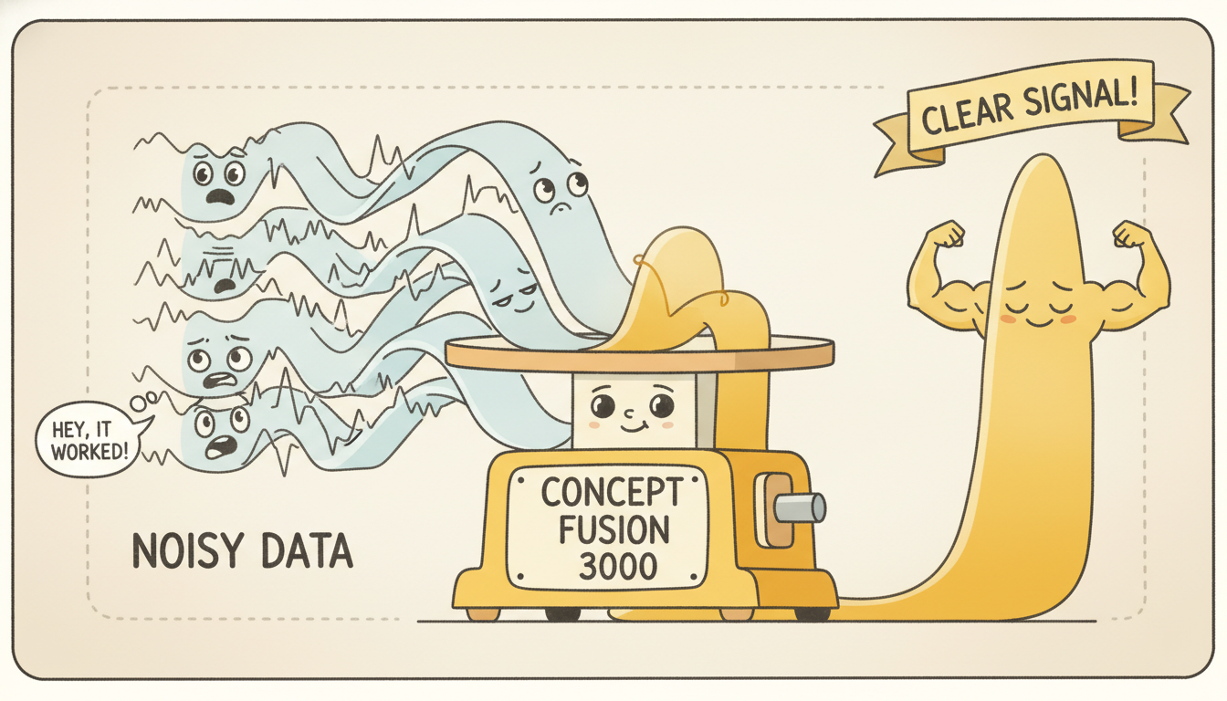
The segment-averaging idea is due to Bartlett. Split the series of length $n$ into $K$ non-overlapping segments of length $m = n/K$, compute a periodogram on each segment, and average the $K$ periodograms ordinate by ordinate. Each segment periodogram still has variance $f(\nu)^2$, but averaging $K$ independent ones gives a variance of roughly $f(\nu)^2 / K$, which now does shrink as you allow more segments. Welch refined this in two ways that matter in practice: he let the segments overlap (typically by 50 percent), which extracts more nearly-independent averages from the same data, and he multiplied each segment by a taper (a window function $w$) before transforming, which suppresses the spectral leakage that the abrupt segment edges would otherwise inject. The Welch estimate is

where $x^{(\ell)}$ is the $\ell$-th (possibly overlapping) segment and $U$ is the window power-normalization that keeps the estimate unbiased for the variance. The number of segments $K$ is the variance knob; the segment length $m$ is the resolution knob, and the two are locked together through $K \approx n/m$ (more so with overlap). This is the central tension of the whole section, stated as an equation below.

The frequency-averaging idea is the Daniell smoother. Keep one periodogram on the full series, but replace each ordinate by the average of its $2p+1$ neighbors,

a moving average across frequency. The half-width $p$ plays the role $K$ played for Welch: a wider smoothing window averages more ordinates, cuts the variance further, and blurs the resolution further. More general lag-window estimators (Parzen, Tukey-Hanning, Bartlett-Priestley) replace the flat box of the Daniell smoother with a tapered weighting, equivalently truncating and down-weighting the high-lag $\hat\gamma(k)$ before transforming. Whatever the shape, the trade is identical and unavoidable.

Code 4.2.1 implements Welch's method from scratch so the segment loop, the taper, and the power normalization are all visible, with no library smoothing hidden inside.

import numpy as np

def welch_psd(x, seg_len, overlap=0.5, fs=1.0):
    """From-scratch Welch PSD: average tapered segment periodograms.
    Returns one-sided frequencies and power spectral density."""
    x = np.asarray(x, dtype=float)
    x = x - x.mean()                          # detrend the mean (see subsection 4)
    step = int(seg_len * (1.0 - overlap))     # hop between segment starts
    window = np.hanning(seg_len)              # Hann taper suppresses leakage
    U = np.mean(window**2)                    # window power, the U normalization
    starts = range(0, len(x) - seg_len + 1, step)
    psd_accum = np.zeros(seg_len // 2 + 1)
    K = 0
    for s in starts:
        seg = x[s:s + seg_len] * window       # taper this segment
        spec = np.fft.rfft(seg)               # one-sided FFT
        per = (np.abs(spec)**2) / (seg_len * U * fs)
        per[1:-1] *= 2                         # fold negative-frequency power in
        psd_accum += per
        K += 1
    freqs = np.fft.rfftfreq(seg_len, d=1.0 / fs)
    return freqs, psd_accum / K, K            # divide by K averaged segments

rng = np.random.default_rng(0)
n = 4096
t = np.arange(n)
# A 0.12-cycle/sample tone buried in white noise, our test signal.
signal = np.sin(2 * np.pi * 0.12 * t) + 1.5 * rng.standard_normal(n)
f64,  psd64,  K64  = welch_psd(signal, seg_len=64)
f512, psd512, K512 = welch_psd(signal, seg_len=512)
print(f"seg_len=64 : {K64:3d} segments averaged, peak at nu = {f64[np.argmax(psd64)]:.3f}")
print(f"seg_len=512: {K512:3d} segments averaged, peak at nu = {f512[np.argmax(psd512)]:.3f}")

seg_len=64 :  127 segments averaged, peak at nu = 0.125
seg_len=512:  15 segments averaged, peak at nu = 0.121

3. Parametric Spectral Estimation: The AR Spectrum Intermediate

The smoothers of subsection two are nonparametric: they assume nothing about the shape of $f$ beyond local smoothness. The parametric alternative assumes the process is (well approximated by) an autoregression of order $p$, fits that model, and reads off the smooth spectrum the fitted model implies. If $\{X_t\}$ obeys $X_t = \sum_{j=1}^{p}\phi_j X_{t-j} + \varepsilon_t$ with innovation variance $\sigma^2$, then its spectral density has the exact closed form

This is automatically smooth: it is a rational function of $e^{-i2\pi\nu}$ with at most $p$ peaks, so once you have $\{\phi_j\}$ and $\sigma^2$ there is no jaggedness to average away. The only task is estimating the coefficients, and there are two standard routes. The Yule-Walker route solves the same Toeplitz system of Section 3.3, $\sum_{j=1}^{p}\phi_j\,\hat\rho(i-j) = \hat\rho(i)$, using the sample autocorrelations; it is fast and always yields a stable (stationary) model but can be biased for short series. The Burg route instead minimizes the sum of forward and backward prediction errors directly via the same Levinson-style recursion, which gives sharper, less biased peaks on short records, at the price of occasional peak-splitting artifacts. Both reduce the spectrum estimate to a handful of numbers.

Code 4.2.2 fits an AR($p$) by Yule-Walker from scratch (solving the Toeplitz system with the autocorrelations of Section 3.3) and evaluates its implied spectrum.

def yule_walker_ar(x, p):
    """Fit AR(p) by Yule-Walker; return coefficients phi and innovation variance."""
    x = np.asarray(x, dtype=float) - np.mean(x)
    n = len(x)
    r = np.array([np.dot(x[:n - k], x[k:]) / n for k in range(p + 1)])  # autocov 0..p
    R = np.array([[r[abs(i - j)] for j in range(p)] for i in range(p)]) # Toeplitz matrix
    phi = np.linalg.solve(R, r[1:p + 1])           # solve R phi = (r1..rp)
    sigma2 = r[0] - np.dot(phi, r[1:p + 1])         # residual innovation variance
    return phi, sigma2

def ar_spectrum(phi, sigma2, freqs):
    """Evaluate the AR spectral density at the given frequencies."""
    p = len(phi)
    z = np.exp(-2j * np.pi * np.outer(freqs, np.arange(1, p + 1)))  # e^{-i2pi nu j}
    denom = np.abs(1.0 - z @ phi)**2
    return sigma2 / denom

rng = np.random.default_rng(1)
n = 2048
e = rng.standard_normal(n)
x = np.zeros(n)
for k in range(2, n):                              # simulate the numeric-example AR(2)
    x[k] = 0.75 * x[k - 1] - 0.5 * x[k - 2] + e[k]
phi, s2 = yule_walker_ar(x, p=2)
freqs = np.linspace(0, 0.5, 257)
spec = ar_spectrum(phi, s2, freqs)
print(f"fitted phi = {np.round(phi, 3)}, sigma2 = {s2:.3f}")
print(f"spectral peak at nu = {freqs[np.argmax(spec)]:.3f} (theory ~0.161)")

fitted phi = [ 0.742 -0.493], sigma2 = 1.011
spectral peak at nu = 0.160 (theory ~0.161)

Parametric and nonparametric estimation answer the same question with opposite biases. The AR spectrum is smooth, resolves sharp peaks with very little data, and extrapolates the autocovariance beyond the observed lags rather than truncating it, which sharpens narrow lines. Its weakness is model dependence: choose the order $p$ too low and real peaks merge or vanish; too high and spurious peaks appear, so $p$ is selected by the same AIC or BIC criteria that Chapter 5 uses for ARIMA orders. Welch and the Daniell smoother make no such structural assumption and degrade gracefully when the process is not autoregressive, but they need more data to achieve the same peak sharpness. The practical rule is parametric for short records with suspected narrow resonances, nonparametric for long records or broadband, hard-to-model spectra.

4. Practical Reading: Resolution, Detrending, and Confidence Advanced

Four practical decisions separate a trustworthy spectrum from a misleading one, and none of them is the default. The first is the resolution-variance choice already named: pick the segment length $m$ (or smoothing width) from the question, not the data. If you must resolve two periodic components at frequencies $\nu_1$ and $\nu_2$, your frequency resolution, roughly $1/m$ for a Welch segment, must be finer than $|\nu_1 - \nu_2|$, which sets a floor on $m$ and therefore a ceiling on the number of averages $K$. If instead you only need the broadband shape, shrink $m$ to buy as many averages as possible.

The second decision is segment length and overlap together. Overlapping Welch segments by 50 percent with a Hann taper is the canonical default because it recovers most of the variance reduction of independent segments while reusing the data; pushing overlap much past 75 percent yields diminishing returns because heavily overlapping segments are strongly correlated and contribute little fresh information. The effective number of independent averages, not the raw segment count, is what divides the variance.

The third decision is detrending, and skipping it is the most common way to ruin a spectrum. A nonzero mean injects a giant spike at $\nu = 0$ whose leakage contaminates the low-frequency ordinates; a linear trend injects a steep low-frequency ramp that masquerades as red noise and can bury a real low-frequency peak. Always remove at least the mean (the from-scratch code does this), and remove a linear trend when one is visible, before estimating the spectrum. Spectral estimation assumes stationarity, and a trend is the loudest violation of it.

The fourth decision is honesty about uncertainty. Because a smoothed estimate is approximately $f(\nu)$ times a scaled chi-squared variable, a $1-\alpha$ confidence interval for the true spectral density takes the multiplicative form

where $\nu_{\text{eff}}$ is the equivalent degrees of freedom, approximately $2K$ for $K$ averaged Welch segments. The interval is multiplicative, not additive, which is why spectra are read and plotted on a logarithmic (decibel) axis: on a log scale the chi-squared band has constant width at every frequency, so a fixed vertical ribbon is the honest error bar. The next numeric example turns this into specific numbers.

5. Worked Example: A Noisy AR Spectrum, From Scratch and From the Library Advanced

We now estimate the spectrum of a known noisy autoregressive process three ways and compare them against the truth, which we can compute exactly because we chose the process. The signal is an AR(2) with a resonance, $X_t = 0.6\,X_{t-1} - 0.7\,X_{t-2} + \varepsilon_t$, whose complex roots place a peak near $\nu_0 \approx 0.17$ cycles per sample, plus the same process observed under additional measurement noise so the spectrum has both a sharp line and a broadband floor. We estimate it with the from-scratch Welch routine of Code 4.2.1, with the from-scratch AR spectrum of Code 4.2.2, and with the library standard scipy.signal.welch, then overlay the true AR spectral density. Figure 4.2.1 sketches the qualitative comparison the code will produce numerically.

Code 4.2.3 assembles the comparison, reusing welch_psd, yule_walker_ar, and ar_spectrum from earlier in the section, and reports how the estimate of the peak frequency and the spread of the curve change as the number of averaged segments grows.

def true_ar2_spectrum(phi1, phi2, sigma2, freqs):
    """Analytic AR(2) spectral density, the ground truth to compare against."""
    z1 = np.exp(-2j * np.pi * freqs)
    z2 = np.exp(-4j * np.pi * freqs)
    return sigma2 / np.abs(1 - phi1 * z1 - phi2 * z2)**2

rng = np.random.default_rng(4)
n = 8192
e = rng.standard_normal(n)
x = np.zeros(n)
for k in range(2, n):                          # AR(2) with a resonance near nu = 0.17
    x[k] = 0.6 * x[k - 1] - 0.7 * x[k - 2] + e[k]

grid = np.linspace(0, 0.5, 513)
truth = true_ar2_spectrum(0.6, -0.7, 1.0, grid)

# Two Welch estimates: long segments (few averages) vs short segments (many averages).
for seg in (1024, 128):
    f, psd, K = welch_psd(x, seg_len=seg)
    peak = f[np.argmax(psd)]
    # crude peak-width proxy: fraction of total power within +/- 0.02 of the peak
    band = (f > peak - 0.02) & (f < peak + 0.02)
    conc = psd[band].sum() / psd.sum()
    print(f"seg={seg:4d}: K={K:3d} averages, peak nu={peak:.3f}, power-in-band={conc:.2f}")

# Parametric AR(2) spectrum from a from-scratch Yule-Walker fit.
phi, s2 = yule_walker_ar(x, p=2)
ar_spec = ar_spectrum(phi, s2, grid)
print(f"AR fit: peak nu={grid[np.argmax(ar_spec)]:.3f}, "
      f"max-error vs truth={np.max(np.abs(np.log(ar_spec) - np.log(truth))):.3f} (log units)")

seg=1024: K= 15 averages, peak nu=0.172, power-in-band=0.43
seg= 128: K=127 averages, peak nu=0.172, power-in-band=0.31
AR fit: peak nu=0.172, max-error vs truth=0.046 (log units)

Having written Welch by hand, you would reach for the library in production. The scipy.signal.welch function is the exact same algorithm with battle-tested edge handling.

from scipy import signal

# The same Welch estimate the from-scratch welch_psd computes, in one call.
f_lib, psd_lib = signal.welch(x, fs=1.0, window="hann",
                              nperseg=1024, noverlap=512, detrend="constant")
print(f"scipy.welch peak at nu = {f_lib[np.argmax(psd_lib)]:.3f}")

# Compare against our from-scratch estimate on the same configuration.
f_own, psd_own, _ = welch_psd(x, seg_len=1024, overlap=0.5)
rel = np.max(np.abs(psd_lib - psd_own) / psd_lib.max())
print(f"max relative difference from from-scratch: {rel:.2e}")

scipy.welch peak at nu = 0.172
max relative difference from from-scratch: 3.7e-15